Introduction
In a previous post I showed how to construct a PMMH pMCMC algorithm for parameter estimation with partially observed Markov processes. The inner loop of a pMCMC algorithm consists of running a particle filter to construct an unbiased estimate of marginal likelihood. This inner loop is the place where the code spends almost all of its time, and so speeding up the particle filter will result in dramatic speedup of the pMCMC algorithm. This is fortunate, since as previously discussed, MCMC algorithms are difficult to parallelise other than on a per iteration basis. Here, each iteration can be speeded up if we can effectively parallelise a particle filter. Particle filters are much easier to parallelise than MCMC algorithms, and so it is tempting to try and exploit this within R. In fact, although it is the case that it is possible to effectively parallelise particle filters in efficient languages using low-level parallelisation tools (say, using C with MPI, or Java concurrency tools), it is not so easy to speed up R-based particle filters using R’s high-level parallelisation constructs, as we shall see.
Particle filters
In the previous post we looked at the function pfMLLik within the CRAN package smfsb. As a reminder, the source code is
pfMLLik <- function (n, simx0, t0, stepFun, dataLik, data)
{
    times = c(t0, as.numeric(rownames(data)))
    deltas = diff(times)
    return(function(...) {
        xmat = simx0(n, t0, ...)
        ll = 0
        for (i in 1:length(deltas)) {
            xmat = t(apply(xmat, 1, stepFun, t0 = times[i], deltat = deltas[i], ...))
            w = apply(xmat, 1, dataLik, t = times[i + 1], y = data[i,], log = FALSE, ...)
            if (max(w) < 1e-20) {
                warning("Particle filter bombed")
                return(-1e+99)
            }
            ll = ll + log(mean(w))
            rows = sample(1:n, n, replace = TRUE, prob = w)
            xmat = xmat[rows, ]
        }
        ll
    })
}
The function itself doesn’t actually run a particle filter, but instead returns a function closure which does (see the previous post for a discussion of lexical scope and function closures in R). There are obviously several different steps within the particle filter, and several of these are amenable to parallelisation. However, for complex models, forward simulation from the model will be the rate-limiting step, where the vast majority of CPU cycles will be spent. Line 9 in the above code is where forward simulation takes place, and in particular, the key function call is the apply call:
apply(xmat, 1, stepFun, t0 = times[i], deltat = deltas[i], ...)
This call applies the forward simulation algorithm stepFun to each row of the matrix xmat independently. Since there are no dependencies between the function calls, this is in principle very straightforward to parallelise on multicore hardware.
Multicore support in R
I’m writing this post on a laptop with an Intel i7 quad core chip, running the 64 bit version of Ubuntu 11.10. R has support for multicore processing on this platform – it is just a simple matter of installing the relevant packages. However, things are changing rapidly regarding multicore support in R right now, so YMMV. Ubuntu 11.10 has R 2.13 by default, but the multicore support is slightly different in the recently released R 2.14. I’m still using R 2.13. I may update this post (or comment) when I move to R 2.14. The main difference is that the package multicore has been replaced by the package parallel. There are a few other minor changes, but it should be easy to adapt what is presented here to 2.14.
There is a new O’Reilly book called Parallel R. I’ve got a copy of it. It does cover the new parallel package in R 2.14, as well as other parallel R topics, but the book is a bit light weight, to say the least, and I reviewed it on this blog. Please read my review for further details before you buy it.
If you haven’t used multicore in R previously, then
install.packages(c("multicore","doMC"))
should get you started (again, I’m assuming that your R version is strictly < 2.14). You can test it has worked with:
library(multicore)
multicore:::detectCores()
When I do this, I get the answer 8 (I have 4 cores, each of which is hyper-threaded). To begin with, I want to tell R to use just 4 process threads, and I can do this with
library(doMC)
registerDoMC(4)
Replacing the second line with registerDoMC() will set things up to use all detected cores (in my case, 8). There are a couple of different strategies we could use to parallelise this. One strategy for parallelising the apply call discussed above is to be to replace it with a foreach / %dopar% loop. This is best illustrated by example. Start with line 9 from the function pfMLLik:
xmat = t(apply(xmat, 1, stepFun, t0 = times[i], deltat = deltas[i], ...))
We can produce a parallelised version by replacing this line with the following block of code:
res=foreach(j=1:dim(xmat)[1]) %dopar% {
  stepFun(xmat[j,], t0 = times[i], deltat = deltas[i], ...)
}
xmat=t(sapply(res,cbind))
Each iteration of the foreach loop is executed independently (possibly using multiple cores), and the result of each iteration is returned as a list, and captured in res. This list of return vectors is then coerced back into a matrix with the final line.
In fact, we can improve on this by using the .combine argument to foreach, which describes how to combine the results from each iteration. Here we can just use rbind to combine the results into a matrix, using:
xmat=foreach(j=1:dim(xmat)[1], .combine="rbind") %dopar% {
  stepFun(xmat[j,], t0 = times[i], deltat = deltas[i], ...)
}
This code is much neater, and in principle ought to be a bit faster, though I haven’t noticed much difference in practice.
In fact, it is not necessary to use the foreach construct at all. The multicore package provides the mclapply function, which is a multicore version of lapply. To use mclapply (or, indeed, lapply) here, we first need to split our matrix into a list of rows, which we can do using the split command. So in fact, our apply call can be replaced with the single line:
xmat=t(sapply(mclapply(split(xmat,row(xmat)), stepFun, t0=times[i], deltat=deltas[i], ...),cbind))
This is actually a much cleaner solution than the method using foreach, but it does require grokking a bit more R. Note that mclapply uses a different method to specify the number of threads to use than foreach/doMC. Here you can either use the named argument to mclapply, mc.cores, or use options(), eg. options(cores=4).
As well as being much cleaner, I find that the mclapply approach is much faster than the foreach/dopar approach for this problem. I’m guessing that this is because foreach doesn’t pre-schedule tasks by default, whereas mclapply does, but I haven’t had a chance to dig into this in detail yet.
A parallelised particle filter
We can now splice the parallelised forward simulation step (using mclapply) back into our particle filter function to get:
require(multicore)
pfMLLik <- function (n, simx0, t0, stepFun, dataLik, data)
{
    times = c(t0, as.numeric(rownames(data)))
    deltas = diff(times)
    return(function(...) {
        xmat = simx0(n, t0, ...)
        ll = 0
        for (i in 1:length(deltas)) {
        xmat=t(sapply(mclapply(split(xmat,row(xmat)), stepFun, t0=times[i], deltat=deltas[i], ...),cbind))
            w = apply(xmat, 1, dataLik, t = times[i + 1], y = data[i,], log = FALSE, ...)
            if (max(w) < 1e-20) {
                warning("Particle filter bombed")
                return(-1e+99)
            }
            ll = ll + log(mean(w))
            rows = sample(1:n, n, replace = TRUE, prob = w)
            xmat = xmat[rows, ]
        }
        ll
    })
}
This can be used in place of the version supplied with the smfsb package for slow simulation algorithms running on modern multicore machines.
There is an issue regarding Monte Carlo simulations such as this and the multicore package (whether you use mclapply or foreach/dopar) in that it adopts a “different seeds” approach to parallel random number generation, rather than a true parallel random number generator. This probably isn’t worth worrying too much about now, since it is fixed in the new parallel package in R 2.14, but is something to be aware of. I discuss parallel random number generation issues in Wilkinson (2005).
Granularity
The above code is now a parallel particle filter, and can now be used in place of the serial version that is part of the smfsb package. However, if you try it out on a simple example, you will most likely be disappointed. In particular, if you use it for the pMCMC example discussed in the previous post, you will see that the parallel version of the example actually runs much slower than the serial version (at least, it does for me). However, that is because the forward simulator stepFun, used in that example, was actually a very fast simulation algorithm, stepLVc, written in C. In this case, the overhead of setting up and closing down the threads, and distributing the tasks, and collating the results from the worker threads back in the master thread, etc., outweighs the advantage of running the individual tasks in parallel. This is why parallel programming is difficult. What is needed here is for the individual tasks to be sufficiently computationally intensive that the overheads associated with parallelisation are easily outweighed by the ability to run the tasks in parallel. In the context of particle filtering, this is particularly problematic, as if the forward simulator is very slow, running a reasonable particle filter is going to be very, very slow, and then you probably don’t want to be working in R anyway… Parallelising a particle filter written in C using MPI is much more likely to be successful, as it offers much more fine grained control of exactly how the tasks and processes are managed, but at the cost of increased development time. In a previous post I gave an introduction to parallel Monte Carlo with C and MPI, and I’ve written more extensively about parallel MCMC in Wilkinson (2005). It also looks as though the new parallel package in R 2.14 offers more control of parallelisation, so that also might help. However, if you are using a particle filter as part of a pMCMC algorithm, there is another strategy you can use at a higher level of granularity which might be useful even within R in some situations.
Multiple particle filters and pMCMC
Let’s look again at the main loop of the pMCMC algorithm discussed in the previous post:
for (i in 1:iters) {
	message(paste(i,""),appendLF=FALSE)
	for (j in 1:thin) {
		thprop=th*exp(rnorm(p,0,tune))
		llprop=mLLik(thprop)
		if (log(runif(1)) < llprop - ll) {
			th=thprop
			ll=llprop
			}
		}
	thmat[i,]=th
	}
It is clear that the main computational bottleneck of this code is the call to mLLik on line 5, as this is the call which runs the particle filter. The purpose of making the call is to obtain an unbiased estimate of marginal likelihood. However, there are plenty of other ways that we can obtain such estimates than by running a single particle filter. In particular, we could run multiple particle filters and average the results. So, let’s look at how to do this in the multicore setting. Let’s start by thinking about running 4 particle filters. We could just replace the line
llprop=mLLik(thprop)
with the code
llprop=0.25*foreach(i=1:4, .combine="+") %dopar% {
    mLLik(thprop)
    }
Now, there are at least 2 issues with this. The first is that we are now just running 4 particle filters rather than 1, and so even with perfect parallelisation, it will run no quicker than the code we started with. However, the idea is that by running 4 particle filters we ought to be able to get away with each particle filter using fewer particles, though it isn’t trivial to figure out exactly how many. For example, averaging the results from 4 particle filters, each of which uses 25 particles is not as good as running a single particle filter with 100 particles. In practice, some trial and error is likely to be required. The second problem is that we have computed the mean of the log of the likelihoods, and not the likelihoods themselves. This will almost certainly work fine in practice, as the resulting estimate will in most cases be very close to unbiased, but it will not be exactly unbiased, as so will not lead to an “exact” approximate algorithm. In principle, this can be fixed by instead using
res=foreach(i=1:4) %dopar% {
    mLLik(thprop)
    }
llprop=log(mean(sapply(res,exp)))
but in practice this is likely to be subject to numerical underflow problems, as it involves manipulating raw likelihood values, which is generally a bad idea. It is possible to compute the log of the mean of the likelihoods in a more numerically stable way, but that is left as an exercise for the reader, as this post is way too long already… However, one additional tip worth mentioning is that the foreach package includes a convenience function called times for situations like the above, where the argument is not varying over calls. So the above code can be replaced with
res=times(4) %dopar% mLLik(thprop)
llprop=log(mean(sapply(res,exp)))
which is a bit cleaner and more readable.
Using this approach to parallelisation, there is now a much better chance of getting some speedup on multicore architectures, as the granularity of the tasks being parallelised is now much larger. Consider the example from the previous post, where at each iteration we ran a particle filter with 100 particles. If we now re-run that example, but instead use 4 particle filters each using 25 particles, we do get a slight speedup. However, on my laptop, the speedup is only around a factor of 1.6 using 4 cores, and as already discussed, 4 filters each with 25 particles isn’t actually quite as good as a single filter with 100 particles anyway. So, the benefits are rather modest here, but will be much better with less trivial examples (slower simulators). For completeness, a complete runnable demo script is included after the references. Also, it is probably worth emphasising that if your pMCMC algorithm has a short burn-in period, you may well get much better overall speed-ups by just running parallel MCMC chains. Depressing, perhaps, but true.
References
McCallum, E., Weston, S. (2011) Parallel R, O’Reilly.
Wilkinson, D. J. (2005) Parallel Bayesian Computation, Chapter 16 in E. J. Kontoghiorghes (ed.) Handbook of Parallel Computing and Statistics, Marcel Dekker/CRC Press, 481-512.
Wilkinson, D. J. (2011) Stochastic Modelling for Systems Biology, second edition, Boca Raton, Florida: Chapman & Hall/CRC Press.
Demo script
require(smfsb)
data(LVdata)
require(multicore)
require(doMC)
registerDoMC(4)
# set up data likelihood
noiseSD=10
dataLik <- function(x,t,y,log=TRUE,...)
{
ll=sum(dnorm(y,x,noiseSD,log=TRUE))
if (log)
return(ll)
else
return(exp(ll))
}
# now define a sampler for the prior on the initial state
simx0 <- function(N,t0,...)
{
mat=cbind(rpois(N,50),rpois(N,100))
colnames(mat)=c("x1","x2")
mat
}
# convert the time series to a timed data matrix
LVdata=as.timedData(LVnoise10)
# create marginal log-likelihood functions, based on a particle filter
# use 25 particles instead of 100
mLLik=pfMLLik(25,simx0,0,stepLVc,dataLik,LVdata)
iters=1000
tune=0.01
thin=10
th=c(th1 = 1, th2 = 0.005, th3 = 0.6)
p=length(th)
ll=-1e99
thmat=matrix(0,nrow=iters,ncol=p)
colnames(thmat)=names(th)
# Main pMCMC loop
for (i in 1:iters) {
message(paste(i,""),appendLF=FALSE)
for (j in 1:thin) {
thprop=th*exp(rnorm(p,0,tune))
res=times(4) %dopar% mLLik(thprop)
llprop=log(mean(sapply(res,exp)))
if (log(runif(1)) < llprop - ll) {
th=thprop
ll=llprop
}
}
thmat[i,]=th
}
message("Done!")
# Compute and plot some basic summaries
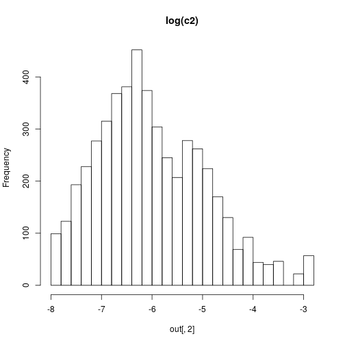
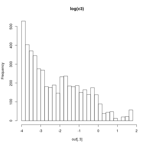
mcmcSummary(thmat)


 of the process is being updated. That is, we target
  (for known, fixed,
  ) rather than
  . This special case is known as the particle independent Metropolis-Hastings (PIMH) sampler.
 using a bootstrap filter, and then accepting the proposal with probability
  , where
  is the
 is the bootstrap filter’s estimate of marginal likelihood for the new path, and
  is the estimate associated with the current path. Again using notation from the
 . Again, be sure to see the previous post for the explanation.
 rather than the exact conditional distribution
![\displaystyle \frac{\tilde{q}(\mathbf{x}_0,\ldots,\mathbf{x}_T,\mathbf{a}_0,\ldots,\mathbf{a}_{T-1})} {\displaystyle p(x_0^{b_0^k})\left[\prod_{t=0}^{T-1} \pi_t^{b_t^k}p\left(x_{t+1}^{b_{t+1}^k}|x_t^{b_t^k}\right)\right]}](https://s0.wp.com/latex.php?latex=%5Cdisplaystyle+%5Cfrac%7B%5Ctilde%7Bq%7D%28%5Cmathbf%7Bx%7D_0%2C%5Cldots%2C%5Cmathbf%7Bx%7D_T%2C%5Cmathbf%7Ba%7D_0%2C%5Cldots%2C%5Cmathbf%7Ba%7D_%7BT-1%7D%29%7D+%7B%5Cdisplaystyle+p%28x_0%5E%7Bb_0%5Ek%7D%29%5Cleft%5B%5Cprod_%7Bt%3D0%7D%5E%7BT-1%7D+%5Cpi_t%5E%7Bb_t%5Ek%7Dp%5Cleft%28x_%7Bt%2B1%7D%5E%7Bb_%7Bt%2B1%7D%5Ek%7D%7Cx_t%5E%7Bb_t%5Ek%7D%5Cright%29%5Cright%5D%7D&bg=ffffff&fg=333333&s=0&c=20201002) .
. paths, of which the conditioned-on trajectory is one.
 be the path that is to be conditioned on, with ancestral lineage
  . Then, for
  , sample
  and set
  . Now suppose that at time
  we have a weighted sample from
  . First resample by sampling
  . Next sample
  . Then for all
  set
set 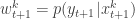 and normalise with
 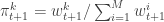 . Propagate this weighted set of particles to the next time point. At time
  select a single trajectory by sampling
  .
. of the
  random variables in the augmented state space at each iteration. Since the block of variables to be updated is random, this defines an ergodic sampler for
  particles, and we have explained why the marginal distribution of the selected trajectory is the exact conditional distribution.
 and the currently sampled path,


 . On the other hand, the PMMH algorithm is an MCMC algorithm which targets the full joint posterior distribution
  ). Below I will describe the algorithm and explain why it works, but first it is necessary to understand the relationship between marginal, joint and “likelihood-free” MCMC updating schemes for such latent variable models.
 is proposed from
  and accepted with probability
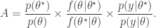
 required in the acceptance ratio is often difficult to compute.
 even when we can’t evaluate it, or marginalise
  is simulated from the model
  . The pair
  is then jointly accepted with ratio
 . The pair
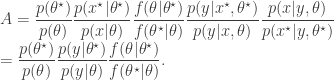
 , as the algorithms above. First, a proposed new
  is accepted using the Metropolis-Hastings ratio
 is the particle filter’s (unbiased) estimate of marginal likelihood, described in the previous post, and below. Note that this approach tends to the perfect joint/marginal updating scheme as the number of particles used in the filter tends to infinity. Note also that for a single particle, the particle filter just blindly forward simulates from
  and that the filter’s estimate of marginal likelihood is just the observed data likelihood
  leading precisely to the simple likelihood-free scheme. To understand for an arbitrary finite number of particles,
  ,
,  ,
,  . Initialise the particle filter with
  , where
  and
and  is undefined). Now suppose at time
  . First resample by sampling
  ,
,  . Here we use
  for the discrete distribution on
  with probability mass function
  . Next sample
  . Set
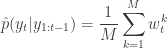
. Set  to the next step… We define the filter’s estimate of likelihood as
 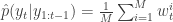 and
and 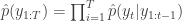 . See
. See ![\displaystyle \tilde{q}(\mathbf{x}_0,\ldots,\mathbf{x}_T,\mathbf{a}_0,\ldots,\mathbf{a}_{T-1}) = \left[\prod_{k=1}^M p(x_0^k)\right] \left[\prod_{t=0}^{T-1} \prod_{k=1}^M \pi_t^{a_t^k} p(x_{t+1}^k|x_t^{a_t^k}) \right]](https://s0.wp.com/latex.php?latex=%5Cdisplaystyle++%5Ctilde%7Bq%7D%28%5Cmathbf%7Bx%7D_0%2C%5Cldots%2C%5Cmathbf%7Bx%7D_T%2C%5Cmathbf%7Ba%7D_0%2C%5Cldots%2C%5Cmathbf%7Ba%7D_%7BT-1%7D%29++%3D+%5Cleft%5B%5Cprod_%7Bk%3D1%7D%5EM+p%28x_0%5Ek%29%5Cright%5D+%5Cleft%5B%5Cprod_%7Bt%3D0%7D%5E%7BT-1%7D++++%5Cprod_%7Bk%3D1%7D%5EM+%5Cpi_t%5E%7Ba_t%5Ek%7D+p%28x_%7Bt%2B1%7D%5Ek%7Cx_t%5E%7Ba_t%5Ek%7D%29+%5Cright%5D++&bg=ffffff&fg=333333&s=0&c=20201002)
 from
from  giving the joint density

 , and
, and  . If we now think about the structure of the PMMH algorithm, our proposal on the space of all random variables in the problem is in fact

 when we consider just the parameters and the selected trajectory. But if we consider the terms in the joint distribution of the proposal corresponding to the trajectory selected by
 ![\displaystyle p_\theta(x_0^{b_0^{k'}})\left[\prod_{t=0}^{T-1} \pi_t^{b_t^{k'}} p_\theta(x_{t+1}^{b_{t+1}^{k'}}|x_t^{b_t^{k'}})\right]\pi_T^{k'} = p_\theta(x_{0:T}^{k'})\prod_{t=0}^T \pi_t^{b_t^{k'}}](https://s0.wp.com/latex.php?latex=%5Cdisplaystyle++p_%5Ctheta%28x_0%5E%7Bb_0%5E%7Bk%27%7D%7D%29%5Cleft%5B%5Cprod_%7Bt%3D0%7D%5E%7BT-1%7D+%5Cpi_t%5E%7Bb_t%5E%7Bk%27%7D%7D++++p_%5Ctheta%28x_%7Bt%2B1%7D%5E%7Bb_%7Bt%2B1%7D%5E%7Bk%27%7D%7D%7Cx_t%5E%7Bb_t%5E%7Bk%27%7D%7D%29%5Cright%5D%5Cpi_T%5E%7Bk%27%7D++%3D++p_%5Ctheta%28x_%7B0%3AT%7D%5E%7Bk%27%7D%29%5Cprod_%7Bt%3D0%7D%5ET+%5Cpi_t%5E%7Bb_t%5E%7Bk%27%7D%7D++&bg=ffffff&fg=333333&s=0&c=20201002)
 in terms of the unnormalised weights, simplifies to
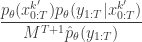
 in the acceptance ratio, we knock out the normalising constant, allowing all of the other terms in the proposal to be marginalised away. In other words, the target of the chain can be written as proportional to

 together with a prior on
  , giving a joint model

 from some fairly arbitrary proposal distribution and then accepting the value with probability
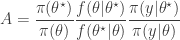
 will still lead to the exact posterior if the estimate is unbiased in the sense that
 ![E[\hat\pi(y|\theta)]=\pi(y|\theta)](https://s0.wp.com/latex.php?latex=E%5B%5Chat%5Cpi%28y%7C%5Ctheta%29%5D%3D%5Cpi%28y%7C%5Ctheta%29&bg=ffffff&fg=333333&s=0&c=20201002) . Consequently, sources of (cheap) unbiased Monte Carlo estimates of (marginal) likelihood are of potential interest in the development of exact MCMC algorithms.
. Consequently, sources of (cheap) unbiased Monte Carlo estimates of (marginal) likelihood are of potential interest in the development of exact MCMC algorithms.

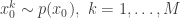
 and simulate realisations from
  . That is, simulate values
  from
from  , and then put
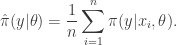
 . That is,
  having the same support as


 . The weights,
  , are known as importance weights.
 using values sampled from an auxiliary distribution
  , where we now supress any dependence of the distributions on model parameters,
  from
from  . Then compute normalised weights
 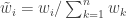 . Generate a new sample of size
  case, the final sample will be exactly drawn from the auxiliary and not the target. The procedure is asymptotic, in that it improves as the sample size increases, tending to the exact target as
  . The proportion of the auxiliary samples falling in a small interval
  will be
  , corresponding to roughly
  particles. The weight for each of those particles will be
  , and since the expected weight of a random particle is 1, the sum of all weights will be (roughly)
 ![\tilde{w}(x)=\pi(x)/[N\pi'(x)]](https://s0.wp.com/latex.php?latex=%5Ctilde%7Bw%7D%28x%29%3D%5Cpi%28x%29%2F%5BN%5Cpi%27%28x%29%5D&bg=ffffff&fg=333333&s=0&c=20201002) . The combined weight of all particles in
. The combined weight of all particles in  . Clearly then, when we resample
  particles from this interval. This corresponds to a proportion
  , corresponding to a density of
  governed by a transition kernel
  is partially observed via some measurement model
  leading to data
  . The idea is to make inference for the hidden states
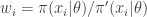
  . The method is a very simple application of the importance resampling technique. At each time,
  .
. with uniform normalised weights
  . Then suppose that we have a weighted sample
  from
from  (giving an approximate random sample from
  . Next propagate each particle forward according to the Markov process model by sampling
  (giving an approximate random sample from
  ). Then for each of the new particles, compute a weight
  .
. 

 . It is much less clear, but nevertheless true that this estimator is also unbiased. The standard reference for this fact is
  . This turns out to be a simple special case of the particle marginal Metropolis-Hastings (PMMH) algorithm described in