The pseudo-marginal approach to “exact approximate” MCMC algorithms

Motivation and background

In this post I will try and explain an important idea behind some recent developments in MCMC theory. First, let me give some motivation. Suppose you are trying to implement a Metropolis-Hastings algorithm, as discussed in a previous post (required reading!), but a key likelihood term needed for the acceptance ratio is difficult to evaluate (most likely it is a marginal likelihood of some sort). If it is possible to obtain a Monte-Carlo estimate for that likelihood term (which it sometimes is, for example, using importance sampling), one could obviously just plug it in to the acceptance ratio and hope for the best. What is not at all obvious is that if your Monte-Carlo estimate satisfies some fairly weak property then the equilibrium distribution of the Markov chain will remain exactly as it would be if the exact likelihood had been available. Furthermore, it is exact even if the Monte-Carlo estimate is very noisy and imprecise (though the mixing of the chain will be poorer in this case). This is the “exact approximate” pseudo-marginal MCMC approach. To give credit where it is due, the idea was first introduced by Mark Beaumont in Beaumont (2003), where he was using an importance sampling based approximate likelihood in the context of a statistical genetics example. This was later picked up by Christophe Andrieu and Gareth Roberts, who studied the technical properties of the approach in Andrieu and Roberts (2009). The idea is turning out to be useful in several contexts, and in particular, underpins the interesting new Particle MCMC algorithms of Andrieu et al (2010), which I will discuss in a future post. I’ve heard Mark, Christophe, Gareth and probably others present this concept, but this post is most strongly inspired by a talk that Christophe gave at the IMS 2010 meeting in Gothenburg this summer.

The pseudo-marginal Metropolis-Hastings algorithm

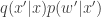
Let’s focus on the simplest version of the problem, where we want to sample from a target using a proposal . As explained previously, the required Metropolis-Hastings acceptance ratio will take the form

Here we are assuming that is difficult to evaluate (usually because it is a marginalised version of some higher-dimensional distribution), but that a Monte-Carlo estimate of , which we shall denote , can be computed. We can obviously just substitute this estimate into the acceptance ratio to get

but it is not immediately clear that in many cases this will lead to the Markov chain having an equilibrium distribution that is exactly . It turns out that it is sufficient that the likelihood estimate, is non-negative, and unbiased, in the sense that , where the expectation is with respect to the Monte-Carlo error for a given fixed value of . In fact, as we shall see, this condition is actually a bit stronger than is really required.

Put , representing the noise in the Monte-Carlo estimate of , and suppose that (note that in an abuse of notation, the function is unrelated to ). The main condition we will assume is that , where is a constant independent of . In the case of , we have the (typical) special case of . For now, we will also assume that , but we will consider relaxing this constraint later.

The key to understanding the pseudo-marginal approach is to realise that at each iteration of the MCMC algorithm a new value of is being proposed in addition to a new value for . If we regard the proposal mechanism as a joint update of and , it is clear that the proposal generates from the density , and we can re-write our “approximate” acceptance ratio as

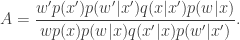
Inspection of this acceptance ratio reveals that the target of the chain must be (proportional to)

This is a joint density for , but the marginal for can be obtained by integrating over the range of with respect to . Using the fact that , this then clearly gives a density proportional to , and this is precisely the target that we require. Note that for this to work, we must keep the old value of from one iteration to the next – that is, we must keep and re-use our noisy value to include in the acceptance ratio for our next MCMC iteration – we should not compute a new Monte-Carlo estimate for the likelihood of the old state of the chain.

Examples

We will consider again the example from the previous post – simulation of a chain with a N(0,1) target using uniform innovations. Using R, the main MCMC loop takes the form

pmmcmc<-function(n=1000,alpha=0.5) 
{
        vec=vector("numeric", n)
        x=0
        oldlik=noisydnorm(x)
        vec[1]=x
        for (i in 2:n) {
                innov=runif(1,-alpha,alpha)
                can=x+innov
                lik=noisydnorm(can)
                aprob=lik/oldlik
                u=runif(1)
                if (u < aprob) { 
                        x=can
                        oldlik=lik
			}
                vec[i]=x
        }
        vec
}

Here we are assuming that we are unable to compute dnorm exactly, but instead only a Monte-Carlo estimate called noisydnorm. We can start with the following implementation

noisydnorm<-function(z)
{
	dnorm(z)*rexp(1,1)
}

Each time this function is called, it will return a non-negative random quantity whose expectation is dnorm(z). We can now run this code as follows.

plot.mcmc<-function(mcmc.out)
{
	op=par(mfrow=c(2,2))
	plot(ts(mcmc.out),col=2)
	hist(mcmc.out,30,col=3)
	qqnorm(mcmc.out,col=4)
	abline(0,1,col=2)
	acf(mcmc.out,col=2,lag.max=100)
	par(op)
}

metrop.out<-pmmcmc(10000,1)
plot.mcmc(metrop.out)

MCMC output and convergence diagnostics

So we see that we have exactly the right N(0,1) target, despite using the (very) noisy noisydnorm function in place of the dnorm function. This noisy likelihood function is clearly unbiased. However, as already discussed, a constant bias in the noise is also acceptable, as the following function shows.

noisydnorm<-function(z)
{
	dnorm(z)*rexp(1,2)
}

Re-running the code with this function also leads to the correct equilibrium distribution for the chain. However, it really does matter that the bias is independent of the state of the chain, as the following function shows.

noisydnorm<-function(z)
{
	dnorm(z)*rexp(1,0.1+10*z*z)
}

Running with this function leads to the wrong equilibrium. However, it is OK for the distribution of the noise to depend on the state, as long as its expectation does not. The following function illustrates this.

noisydnorm<-function(z)
{
	dnorm(z)*rgamma(1,0.1+10*z*z,0.1+10*z*z)
}

This works just fine. So far we have been assuming that our noisy likelihood estimates are non-negative. This is clearly desirable, as otherwise we could wind up with negative Metropolis-Hasting ratios. However, as long as we are careful about exactly what we mean, even this non-negativity condition may be relaxed. The following function illustrates the point.

noisydnorm<-function(z)
{
	dnorm(z)*rnorm(1,1)
}

Despite the fact that this function will often produce negative values, the equilibrium distribution of the chain still seems to be correct! An even more spectacular example follows.

noisydnorm<-function(z)
{
	dnorm(z)*rnorm(1,0)
}

Astonishingly, this one works too, despite having an expected value of zero! However, the following doesn’t work, even though it too has a constant expectation of zero.

noisydnorm<-function(z)
{
	dnorm(z)*rnorm(1,0,0.1+10*z*z)
}

I don’t have time to explain exactly what is going on here, so the precise details are left as an exercise for the reader. Suffice to say that the key requirement is that it is the distribution of W conditioned to be non-negative which must have the constant bias property – something clearly violated by the final noisydnorm example.

Before finishing this post, it is worth re-emphasising the issue of re-using old Monte-Carlo estimates. The following function will not work (exactly), though in the case of good Monte-Carlo estimates will often work tolerably well.

approxmcmc<-function(n=1000,alpha=0.5) 
{
        vec=vector("numeric", n)
        x=0
        vec[1]=x
        for (i in 2:n) {
                innov=runif(1,-alpha,alpha)
                can=x+innov
                lik=noisydnorm(can)
                oldlik=noisydnorm(x)
                aprob=lik/oldlik
                u=runif(1)
                if (u < aprob) { 
                        x=can
			}
                vec[i]=x
        }
        vec
}

In a subsequent post I will show how these ideas can be put into practice in the context of a Bayesian inference example.