approximate – Darren Wilkinson's blog

MCMC code for Bayesian inference for a discretely observed stochastic kinetic model

In June this year the (twice COVID-delayed) Richard J Boys Memorial Workshop finally took place, celebrating the life and work of my former colleague and collaborator, who died suddenly in 2019 (obituary). I completed the programme of talks by delivering the inaugural RSS North East Richard Boys lecture. For this, I decided that it would be most appropriate to talk about the paper Bayesian inference for a discretely observed stochastic kinetic model, published in Statistics and Computing in 2008. The paper is concerned with (exact and approximate) MCMC-based fully Bayesian inference for continuous time Markov jump processes observed partially and discretely in time. Although the ideas are generally applicable to a broad class of “stochastic kinetic models”, the running example throughout the paper is a discrete stochastic Lotka Volterra model.

In preparation for the talk, I managed to track down most of the MCMC codes used for the examples presented in the paper. This included C code I wrote for exact and approximate block-updating algorithms, and Fortran code written by Richard using an exact reversible jump MCMC approach. I’ve fixed up all of the codes so that they are now easy to build and run on a modern Linux (or other Unix-like) system, and provided some minimal documentation. It is all available in a public github repo. Hopefully this will be of some interest or use to a few people.

Summary stats for ABC

Introduction

In the previous post I gave a very brief introduction to ABC, including a simple example for inferring the parameters of a Markov process given some time series observations. Towards the end of the post I observed that there were (at least!) two potential problems with scaling up the simple approach described, one relating to the dimension of the data and the other relating to the dimension of the parameter space. Before moving on to the (to me, more interesting) problem of the dimension of the parameter space, I will briefly discuss the data dimension problem in this post, and provide a couple of references for further reading.

Summary stats

Recall that the simple rejection sampling approach to ABC involves first sampling a candidate parameter $\theta^\star$ from the prior and then sampling a corresponding data set $x^\star$ from the model. This simulated data set is compared with the true data $x$ using some (pseudo-)norm, $\Vert\cdot\Vert$ , and accepting $\theta^\star$ if the simulated data set is sufficiently close to the true data, $\Vert x^\star - x\Vert <\epsilon$ . It should be clear that if we are using a proper norm then as $\epsilon$ tends to zero the distribution of the accepted values tends to the desired posterior distribution of the parameters given the data.

However, smaller choices of $\epsilon$ will lead to higher rejection rates. This will be a particular problem in the context of high-dimensional $x$ , where it is often unrealistic to expect a close match between all components of $x$ and the simulated data $x^\star$ , even for a good choice of $\theta^\star$ . In this case, it makes more sense to look for good agreement between particular aspects of $x$ , such as the mean, or variance, or auto-correlation, depending on the exact problem and context. If we can find a finite set of sufficient statistics, $s(x)$ for $\theta$ , then it should be clear that replacing the acceptance criterion with $\Vert s(x^\star) - s(x)\Vert <\epsilon$ will also lead to a scheme tending to the true posterior as $\epsilon$ tends to zero (assuming a proper norm on the space of sufficient statistics), and will typically be better than the naive method, since the sufficient statistics will be of lower dimension and less “noisy” that the raw data, leading to higher acceptance rates with no loss of information.

Unfortunately for most problems of practical interest it is not possible to find low-dimensional sufficient statistics, and so people in practice use domain knowledge and heuristics to come up with a set of summary statistics, $s(x)$ which they hope will closely approximate sufficient statistics. There is still a question as to how these statistics should be weighted or transformed to give a particular norm. This can be done using theory or heuristics, and some relevant references for this problem are given at the end of the post.

Implementation in R

Let’s now look at the problem from the previous post. Here, instead of directly computing the Euclidean distance between the real and simulated data, we will look at the Euclidean distance between some (normalised) summary statistics. First we will load some packages and set some parameters.

require(smfsb)
require(parallel)
options(mc.cores=4)
data(LVdata)
 
N=1e7
bs=1e5
batches=N/bs
message(paste("N =",N," | bs =",bs," | batches =",batches))

Next we will define some summary stats for a univariate time series – the mean, the (log) variance, and the first two auto-correlations.

ssinit <- function(vec)
{
  ac23=as.vector(acf(vec,lag.max=2,plot=FALSE)$acf)[2:3]
  c(mean(vec),log(var(vec)+1),ac23)
}

Once we have this, we can define some stats for a bivariate time series by combining the stats for the two component series, along with the cross-correlation between them.

ssi <- function(ts)
{
  c(ssinit(ts[,1]),ssinit(ts[,2]),cor(ts[,1],ts[,2]))
}

This gives a set of summary stats, but these individual statistics are potentially on very different scales. They can be transformed and re-weighted in a variety of ways, usually on the basis of a pilot run which gives some information about the distribution of the summary stats. Here we will do the simplest possible thing, which is to normalise the variance of the stats on the basis of a pilot run. This is not at all optimal – see the references at the end of the post for a description of better methods.

message("Batch 0: Pilot run batch")
prior=cbind(th1=exp(runif(bs,-6,2)),th2=exp(runif(bs,-6,2)),th3=exp(runif(bs,-6,2)))
rows=lapply(1:bs,function(i){prior[i,]})
samples=mclapply(rows,function(th){simTs(c(50,100),0,30,2,stepLVc,th)})
sumstats=mclapply(samples,ssi)
sds=apply(sapply(sumstats,c),1,sd)
print(sds)

# now define a standardised distance
ss<-function(ts)
{
  ssi(ts)/sds
}

ss0=ss(LVperfect)

distance <- function(ts)
{
  diff=ss(ts)-ss0
  sum(diff*diff)
}

Now we have a normalised distance function defined, we can proceed exactly as before to obtain an ABC posterior via rejection sampling.

post=NULL
for (i in 1:batches) {
  message(paste("batch",i,"of",batches))
  prior=cbind(th1=exp(runif(bs,-6,2)),th2=exp(runif(bs,-6,2)),th3=exp(runif(bs,-6,2)))
  rows=lapply(1:bs,function(i){prior[i,]})
  samples=mclapply(rows,function(th){simTs(c(50,100),0,30,2,stepLVc,th)})
  dist=mclapply(samples,distance)
  dist=sapply(dist,c)
  cutoff=quantile(dist,1000/N,na.rm=TRUE)
  post=rbind(post,prior[dist<cutoff,])
}
message(paste("Finished. Kept",dim(post)[1],"simulations"))

Having obtained the posterior, we can use the following code to plot the results.

th=c(th1 = 1, th2 = 0.005, th3 = 0.6)
op=par(mfrow=c(2,3))
for (i in 1:3) {
  hist(post[,i],30,col=5,main=paste("Posterior for theta[",i,"]",sep=""))
  abline(v=th[i],lwd=2,col=2)
}
for (i in 1:3) {
  hist(log(post[,i]),30,col=5,main=paste("Posterior for log(theta[",i,"])",sep=""))
  abline(v=log(th[i]),lwd=2,col=2)
}
par(op)

This gives the plot shown below. From this we can see that the ABC posterior obtained here is very similar to that obtained in the previous post using the full data. Here the dimension reduction is not that great – reducing from 32 data points to 9 summary statistics – and so the improvement in performance is not that noticable. But in higher dimensional problems reducing the dimension of the data is practically essential.

Summary and References

As before, I recommend the wikipedia article on approximate Bayesian computation for further information and a comprehensive set of references for further reading. Here I just want to highlight two references particularly relevant to the issue of summary statistics. It is quite difficult to give much practical advice on how to construct good summary statistics, but how to transform a set of summary stats in a “good” way is a problem that is reasonably well understood. In this post I did something rather naive (normalising the variance), but the following two papers describe much better approaches.

Blum, M. G. B., et al. “A comparative review of dimension reduction methods in approximate Bayesian computation.” Statistical Science 28.2 (2013): 189-208.
Fearnhead, Paul, and Dennis Prangle. “Constructing summary statistics for approximate Bayesian computation: semi‐automatic approximate Bayesian computation.” Journal of the Royal Statistical Society: Series B (Statistical Methodology) 74.3 (2012): 419-474.

I still haven’t addressed the issue of a high-dimensional parameter space – that will be the topic of a subsequent post.

The complete R script

require(smfsb)
require(parallel)
options(mc.cores=4)
data(LVdata)
 
N=1e6
bs=1e5
batches=N/bs
message(paste("N =",N," | bs =",bs," | batches =",batches))
 
ssinit <- function(vec)
{
  ac23=as.vector(acf(vec,lag.max=2,plot=FALSE)$acf)[2:3]
  c(mean(vec),log(var(vec)+1),ac23)
}

ssi <- function(ts)
{
  c(ssinit(ts[,1]),ssinit(ts[,2]),cor(ts[,1],ts[,2]))
}

message("Batch 0: Pilot run batch")
prior=cbind(th1=exp(runif(bs,-6,2)),th2=exp(runif(bs,-6,2)),th3=exp(runif(bs,-6,2)))
rows=lapply(1:bs,function(i){prior[i,]})
samples=mclapply(rows,function(th){simTs(c(50,100),0,30,2,stepLVc,th)})
sumstats=mclapply(samples,ssi)
sds=apply(sapply(sumstats,c),1,sd)
print(sds)

# now define a standardised distance
ss<-function(ts)
{
  ssi(ts)/sds
}

ss0=ss(LVperfect)

distance <- function(ts)
{
  diff=ss(ts)-ss0
  sum(diff*diff)
}

post=NULL
for (i in 1:batches) {
  message(paste("batch",i,"of",batches))
  prior=cbind(th1=exp(runif(bs,-6,2)),th2=exp(runif(bs,-6,2)),th3=exp(runif(bs,-6,2)))
  rows=lapply(1:bs,function(i){prior[i,]})
  samples=mclapply(rows,function(th){simTs(c(50,100),0,30,2,stepLVc,th)})
  dist=mclapply(samples,distance)
  dist=sapply(dist,c)
  cutoff=quantile(dist,1000/N,na.rm=TRUE)
  post=rbind(post,prior[dist<cutoff,])
}
message(paste("Finished. Kept",dim(post)[1],"simulations"))

# plot the results
th=c(th1 = 1, th2 = 0.005, th3 = 0.6)
op=par(mfrow=c(2,3))
for (i in 1:3) {
  hist(post[,i],30,col=5,main=paste("Posterior for theta[",i,"]",sep=""))
  abline(v=th[i],lwd=2,col=2)
}
for (i in 1:3) {
  hist(log(post[,i]),30,col=5,main=paste("Posterior for log(theta[",i,"])",sep=""))
  abline(v=log(th[i]),lwd=2,col=2)
}
par(op)

Introduction to Approximate Bayesian Computation (ABC)

Many of the posts in this blog have been concerned with using MCMC based methods for Bayesian inference. These methods are typically “exact” in the sense that they have the exact posterior distribution of interest as their target equilibrium distribution, but are obviously “approximate”, in that for any finite amount of computing time, we can only generate a finite sample of correlated realisations from a Markov chain that we hope is close to equilibrium.

Approximate Bayesian Computation (ABC) methods go a step further, and generate samples from a distribution which is not the true posterior distribution of interest, but a distribution which is hoped to be close to the real posterior distribution of interest. There are many variants on ABC, and I won’t get around to explaining all of them in this blog. The wikipedia page on ABC is a good starting point for further reading. In this post I’ll explain the most basic rejection sampling version of ABC, and in a subsequent post, I’ll explain a sequential refinement, often referred to as ABC-SMC. As usual, I’ll use R code to illustrate the ideas.

Basic idea

There is a close connection between “likelihood free” MCMC methods and those of approximate Bayesian computation (ABC). To keep things simple, consider the case of a perfectly observed system, so that there is no latent variable layer. Then there are model parameters $\theta$ described by a prior $\pi(\theta)$ , and a forwards-simulation model for the data $x$ , defined by $\pi(x|\theta)$ . It is clear that a simple algorithm for simulating from the desired posterior $\pi(\theta|x)$ can be obtained as follows. First simulate from the joint distribution $\pi(\theta,x)$ by simulating $\theta^\star\sim\pi(\theta)$ and then $x^\star\sim \pi(x|\theta^\star)$ . This gives a sample $(\theta^\star,x^\star)$ from the joint distribution. A simple rejection algorithm which rejects the proposed pair unless $x^\star$ matches the true data $x$ clearly gives a sample from the required posterior distribution.

Exact rejection sampling

1. Sample $\theta^\star \sim \pi(\theta^\star)$
2. Sample $x^\star\sim \pi(x^\star|\theta^\star)$
3. If $x^\star=x$ , keep $\theta^\star$ as a sample from $\pi(\theta|x)$ , otherwise reject.
4. Return to step 1.

This algorithm is exact, and for discrete $x$ will have a non-zero acceptance rate. However, in most interesting problems the rejection rate will be intolerably high. In particular, the acceptance rate will typically be zero for continuous valued $x$ .

ABC rejection sampling

The ABC “approximation” is to accept values provided that $x^\star$ is “sufficiently close” to $x$ . In the first instance, we can formulate this as follows.

1. Sample $\theta^\star \sim \pi(\theta^\star)$
2. Sample $x^\star\sim \pi(x^\star|\theta^\star)$
3. If $\Vert x^\star-x\Vert< \epsilon$ , keep $\theta^\star$ as a sample from $\pi(\theta|x)$ , otherwise reject.
4. Return to step 1.

Euclidean distance is usually chosen as the norm, though any norm can be used. This procedure is “honest”, in the sense that it produces exact realisations from

$\theta^\star\big|\Vert x^\star-x\Vert < \epsilon.$

For suitable small choice of $\epsilon$ , this will closely approximate the true posterior. However, smaller choices of $\epsilon$ will lead to higher rejection rates. This will be a particular problem in the context of high-dimensional $x$ , where it is often unrealistic to expect a close match between all components of $x$ and the simulated data $x^\star$ , even for a good choice of $\theta^\star$ . In this case, it makes more sense to look for good agreement between particular aspects of $x$ , such as the mean, or variance, or auto-correlation, depending on the exact problem and context.

In the simplest case, this is done by forming a (vector of) summary statistic(s), $s(x^\star)$ (ideally a sufficient statistic), and accepting provided that $\Vert s(x^\star)-s(x)\Vert<\epsilon$ for some suitable choice of metric and $\epsilon$ . We will return to this issue in a subsequent post.

Inference for an intractable Markov process

I’ll illustrate ABC in the context of parameter inference for a Markov process with an intractable transition kernel: the discrete stochastic Lotka-Volterra model. A function for simulating exact realisations from the intractable kernel is included in the smfsb CRAN package discussed in a previous post. Using pMCMC to solve the parameter inference problem is discussed in another post. It may be helpful to skim through those posts quickly to become familiar with this problem before proceeding.

So, for a given proposed set of parameters, realisations from the process can be sampled using the functions simTs and stepLV (from the smfsb package). We will use the sample data set LVperfect (from the LVdata dataset) as our “true”, or “target” data, and try to find parameters for the process which are consistent with this data. A fairly minimal R script for this problem is given below.

require(smfsb)
data(LVdata)

N=1e5
message(paste("N =",N))
prior=cbind(th1=exp(runif(N,-6,2)),th2=exp(runif(N,-6,2)),th3=exp(runif(N,-6,2)))
rows=lapply(1:N,function(i){prior[i,]})
message("starting simulation")
samples=lapply(rows,function(th){simTs(c(50,100),0,30,2,stepLVc,th)})
message("finished simulation")

distance<-function(ts)
{
  diff=ts-LVperfect
  sum(diff*diff)
}

message("computing distances")
dist=lapply(samples,distance)
message("distances computed")

dist=sapply(dist,c)
cutoff=quantile(dist,1000/N)
post=prior[dist<cutoff,]

op=par(mfrow=c(2,3))
apply(post,2,hist,30)
apply(log(post),2,hist,30)
par(op)

This script should take 5-10 minutes to run on a decent laptop, and will result in histograms of the posterior marginals for the components of $\theta$ and $\log(\theta)$ . Note that I have deliberately adopted a functional programming style, making use of the lapply function for the most computationally intensive steps. The reason for this will soon become apparent. Note that rather than pre-specifying a cutoff $\epsilon$ , I’ve instead picked a quantile of the distance distribution. This is common practice in scenarios where the distance is difficult to have good intuition about. In fact here I’ve gone a step further and chosen a quantile to give a final sample of size 1000. Obviously then in this case I could have just selected out the top 1000 directly, but I wanted to illustrate the quantile based approach.

One problem with the above script is that all proposed samples are stored in memory at once. This is problematic for problems involving large numbers of samples. However, it is convenient to do simulations in large batches, both for computation of quantiles, and also for efficient parallelisation. The script below illustrates how to implement a batch parallelisation strategy for this problem. Samples are generated in batches of size 10^4, and only the best fitting samples are stored before the next batch is processed. This strategy can be used to get a good sized sample based on a more stringent acceptance criterion at the cost of addition simulation time. Note that the parallelisation code will only work with recent versions of R, and works by replacing calls to lapply with the parallel version, mclapply. You should notice an appreciable speed-up on a multicore machine.

require(smfsb)
require(parallel)
options(mc.cores=4)
data(LVdata)

N=1e5
bs=1e4
batches=N/bs
message(paste("N =",N," | bs =",bs," | batches =",batches))

distance<-function(ts)
{
  diff=ts[,1]-LVprey
  sum(diff*diff)
}

post=NULL
for (i in 1:batches) {
  message(paste("batch",i,"of",batches))
  prior=cbind(th1=exp(runif(bs,-6,2)),th2=exp(runif(bs,-6,2)),th3=exp(runif(bs,-6,2)))
  rows=lapply(1:bs,function(i){prior[i,]})
  samples=mclapply(rows,function(th){simTs(c(50,100),0,30,2,stepLVc,th)})
  dist=mclapply(samples,distance)
  dist=sapply(dist,c)
  cutoff=quantile(dist,1000/N)
  post=rbind(post,prior[dist<cutoff,])
}
message(paste("Finished. Kept",dim(post)[1],"simulations"))

op=par(mfrow=c(2,3))
apply(post,2,hist,30)
apply(log(post),2,hist,30)
par(op)

Note that there is an additional approximation here, since the top 100 samples from each of 10 batches of simulations won’t correspond exactly to the top 1000 samples overall, but given all of the other approximations going on in ABC, this one is likely to be the least of your worries.

Now, if you compare the approximate posteriors obtained here with the “true” posteriors obtained in an earlier post using pMCMC, you will see that these posteriors are really quite poor. However, this isn’t a very fair comparison, since we’ve only done 10^5 simulations. Jacking N up to 10^7 gives the ABC posterior below.

ABC posterior from 10^7 iterations — ABC posterior from 10^7 samples

This is a bit better, but really not great. There are two basic problems with the simplistic ABC strategy adopted here, one related to the dimensionality of the data and the other the dimensionality of the parameter space. The most basic problem that we have here is the dimensionality of the data. We have 16 (bivariate) observations, so we want our stochastic simulation to shoot at a point in a 16- or 32-dimensional space. That’s a tough call. The standard way to address this problem is to reduce the dimension of the data by introducing a few carefully chosen summary statistics and then just attempting to hit those. I’ll illustrate this in a subsequent post. The other problem is that often the prior and posterior over the parameters are quite different, and this problem too is exacerbated as the dimension of the parameter space increases. The standard way to deal with this is to sequentially adapt from the prior through a sequence of ABC posteriors. I’ll examine this in a future post as well, once I’ve also posted an introduction to the use of sequential Monte Carlo (SMC) samplers for static problems.

The pseudo-marginal approach to “exact approximate” MCMC algorithms

Motivation and background

In this post I will try and explain an important idea behind some recent developments in MCMC theory. First, let me give some motivation. Suppose you are trying to implement a Metropolis-Hastings algorithm, as discussed in a previous post (required reading!), but a key likelihood term needed for the acceptance ratio is difficult to evaluate (most likely it is a marginal likelihood of some sort). If it is possible to obtain a Monte-Carlo estimate for that likelihood term (which it sometimes is, for example, using importance sampling), one could obviously just plug it in to the acceptance ratio and hope for the best. What is not at all obvious is that if your Monte-Carlo estimate satisfies some fairly weak property then the equilibrium distribution of the Markov chain will remain exactly as it would be if the exact likelihood had been available. Furthermore, it is exact even if the Monte-Carlo estimate is very noisy and imprecise (though the mixing of the chain will be poorer in this case). This is the “exact approximate” pseudo-marginal MCMC approach. To give credit where it is due, the idea was first introduced by Mark Beaumont in Beaumont (2003), where he was using an importance sampling based approximate likelihood in the context of a statistical genetics example. This was later picked up by Christophe Andrieu and Gareth Roberts, who studied the technical properties of the approach in Andrieu and Roberts (2009). The idea is turning out to be useful in several contexts, and in particular, underpins the interesting new Particle MCMC algorithms of Andrieu et al (2010), which I will discuss in a future post. I’ve heard Mark, Christophe, Gareth and probably others present this concept, but this post is most strongly inspired by a talk that Christophe gave at the IMS 2010 meeting in Gothenburg this summer.

The pseudo-marginal Metropolis-Hastings algorithm

Let’s focus on the simplest version of the problem, where we want to sample from a target $p(x)$ using a proposal $q(x'|x)$ . As explained previously, the required Metropolis-Hastings acceptance ratio will take the form

$\displaystyle A=\frac{p(x')q(x|x')}{p(x)q(x'|x)}.$

Here we are assuming that $p(x)$ is difficult to evaluate (usually because it is a marginalised version of some higher-dimensional distribution), but that a Monte-Carlo estimate of $p(x)$ , which we shall denote $r(x)$ , can be computed. We can obviously just substitute this estimate into the acceptance ratio to get

$\displaystyle A=\frac{r(x')q(x|x')}{r(x)q(x'|x)},$

but it is not immediately clear that in many cases this will lead to the Markov chain having an equilibrium distribution that is exactly $p(x)$ . It turns out that it is sufficient that the likelihood estimate, $r(x)$ is non-negative, and unbiased, in the sense that $E(r(x))=p(x)$ , where the expectation is with respect to the Monte-Carlo error for a given fixed value of $x$ . In fact, as we shall see, this condition is actually a bit stronger than is really required.

Put $W=r(x)/p(x)$ , representing the noise in the Monte-Carlo estimate of $p(x)$ , and suppose that $W \sim p(w|x)$ (note that in an abuse of notation, the function $p(w|x)$ is unrelated to $p(x)$ ). The main condition we will assume is that $E(W|x)=c$ , where $c>0$ is a constant independent of $x$ . In the case of $c=1$ , we have the (typical) special case of $E(r(x))=p(x)$ . For now, we will also assume that $W\geq 0$ , but we will consider relaxing this constraint later.

The key to understanding the pseudo-marginal approach is to realise that at each iteration of the MCMC algorithm a new value of $W$ is being proposed in addition to a new value for $x$ . If we regard the proposal mechanism as a joint update of $x$ and $w$ , it is clear that the proposal generates $(x',w')$ from the density $q(x'|x)p(w'|x')$ , and we can re-write our “approximate” acceptance ratio as

$\displaystyle A=\frac{w'p(x')p(w'|x')q(x|x')p(w|x)}{wp(x)p(w|x)q(x'|x)p(w'|x')}.$

Inspection of this acceptance ratio reveals that the target of the chain must be (proportional to)

$p(x)wp(w|x).$

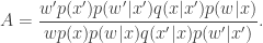
This is a joint density for $(x,w)$ , but the marginal for $x$ can be obtained by integrating over the range of $W$ with respect to $w$ . Using the fact that $E(W|x)=c$ , this then clearly gives a density proportional to $p(x)$ , and this is precisely the target that we require. Note that for this to work, we must keep the old value of $w$ from one iteration to the next – that is, we must keep and re-use our noisy $r(x)$ value to include in the acceptance ratio for our next MCMC iteration – we should not compute a new Monte-Carlo estimate for the likelihood of the old state of the chain.

Examples

We will consider again the example from the previous post – simulation of a chain with a N(0,1) target using uniform innovations. Using R, the main MCMC loop takes the form

pmmcmc<-function(n=1000,alpha=0.5) 
{
        vec=vector("numeric", n)
        x=0
        oldlik=noisydnorm(x)
        vec[1]=x
        for (i in 2:n) {
                innov=runif(1,-alpha,alpha)
                can=x+innov
                lik=noisydnorm(can)
                aprob=lik/oldlik
                u=runif(1)
                if (u < aprob) { 
                        x=can
                        oldlik=lik
			}
                vec[i]=x
        }
        vec
}

Here we are assuming that we are unable to compute dnorm exactly, but instead only a Monte-Carlo estimate called noisydnorm. We can start with the following implementation

noisydnorm<-function(z)
{
	dnorm(z)*rexp(1,1)
}

Each time this function is called, it will return a non-negative random quantity whose expectation is dnorm(z). We can now run this code as follows.

plot.mcmc<-function(mcmc.out)
{
	op=par(mfrow=c(2,2))
	plot(ts(mcmc.out),col=2)
	hist(mcmc.out,30,col=3)
	qqnorm(mcmc.out,col=4)
	abline(0,1,col=2)
	acf(mcmc.out,col=2,lag.max=100)
	par(op)
}

metrop.out<-pmmcmc(10000,1)
plot.mcmc(metrop.out)

So we see that we have exactly the right N(0,1) target, despite using the (very) noisy noisydnorm function in place of the dnorm function. This noisy likelihood function is clearly unbiased. However, as already discussed, a constant bias in the noise is also acceptable, as the following function shows.

noisydnorm<-function(z)
{
	dnorm(z)*rexp(1,2)
}

Re-running the code with this function also leads to the correct equilibrium distribution for the chain. However, it really does matter that the bias is independent of the state of the chain, as the following function shows.

noisydnorm<-function(z)
{
	dnorm(z)*rexp(1,0.1+10*z*z)
}

Running with this function leads to the wrong equilibrium. However, it is OK for the distribution of the noise to depend on the state, as long as its expectation does not. The following function illustrates this.

noisydnorm<-function(z)
{
	dnorm(z)*rgamma(1,0.1+10*z*z,0.1+10*z*z)
}

This works just fine. So far we have been assuming that our noisy likelihood estimates are non-negative. This is clearly desirable, as otherwise we could wind up with negative Metropolis-Hasting ratios. However, as long as we are careful about exactly what we mean, even this non-negativity condition may be relaxed. The following function illustrates the point.

noisydnorm<-function(z)
{
	dnorm(z)*rnorm(1,1)
}

Despite the fact that this function will often produce negative values, the equilibrium distribution of the chain still seems to be correct! An even more spectacular example follows.

noisydnorm<-function(z)
{
	dnorm(z)*rnorm(1,0)
}

Astonishingly, this one works too, despite having an expected value of zero! However, the following doesn’t work, even though it too has a constant expectation of zero.

noisydnorm<-function(z)
{
	dnorm(z)*rnorm(1,0,0.1+10*z*z)
}

I don’t have time to explain exactly what is going on here, so the precise details are left as an exercise for the reader. Suffice to say that the key requirement is that it is the distribution of W conditioned to be non-negative which must have the constant bias property – something clearly violated by the final noisydnorm example.

Before finishing this post, it is worth re-emphasising the issue of re-using old Monte-Carlo estimates. The following function will not work (exactly), though in the case of good Monte-Carlo estimates will often work tolerably well.

approxmcmc<-function(n=1000,alpha=0.5) 
{
        vec=vector("numeric", n)
        x=0
        vec[1]=x
        for (i in 2:n) {
                innov=runif(1,-alpha,alpha)
                can=x+innov
                lik=noisydnorm(can)
                oldlik=noisydnorm(x)
                aprob=lik/oldlik
                u=runif(1)
                if (u < aprob) { 
                        x=can
			}
                vec[i]=x
        }
        vec
}

In a subsequent post I will show how these ideas can be put into practice in the context of a Bayesian inference example.

Tag: approximate