In the previous post I gave a brief introduction to Rainier, a new HMC-based probabilistic programming library/DSL for Scala. In that post I assumed that people were using the latest source version of the library. Since then, version 0.1.1 of the library has been released, so in this post I will demonstrate use of the released version of the software (using the binaries published to Sonatype), and will walk through a slightly more interesting example – a dynamic linear state space model with unknown static parameters. This is similar to, but slightly different from, the DLM example in the Rainier library. So to follow along with this post, all that is required is SBT.
An interactive session
First run SBT from an empty directory, and paste the following at the SBT prompt:
set libraryDependencies  += "com.stripe" %% "rainier-plot" % "0.1.1"
set scalaVersion := "2.12.4"
console
This should give a Scala REPL with appropriate dependencies (rainier-plot has all of the relevant transitive dependencies). We’ll begin with some imports, and then simulating some synthetic data from a dynamic linear state space model with an AR(1) latent state and Gaussian noise on the observations.
import com.stripe.rainier.compute._
import com.stripe.rainier.core._
import com.stripe.rainier.sampler._

implicit val rng = ScalaRNG(1)
val n = 60 // number of observations/time points
val mu = 3.0 // AR(1) mean
val a = 0.95 // auto-regressive parameter
val sig = 0.2 // AR(1) SD
val sigD = 3.0 // observational SD
val state = Stream.
  iterate(0.0)(x => mu + (x - mu) * a + sig * rng.standardNormal).
  take(n).toVector
val obs = state.map(_ + sigD * rng.standardNormal)
Now we have some synthetic data, let’s think about building a probabilistic program for this model. Start with a prior.
case class Static(mu: Real, a: Real, sig: Real, sigD: Real)
val prior = for {
  mu <- Normal(0, 10).param
  a <- Normal(1, 0.1).param
  sig <- Gamma(2,1).param
  sigD <- Gamma(2,2).param
  sp <- Normal(0, 50).param
} yield (Static(mu, a, sig, sigD), List(sp))
Note the use of a case class for wrapping the static parameters. Next, let’s define a function to add a state and associated observation to an existing model.
Given this, we can generate the probabilistic program for our model as a fold over the data initialised with the prior.
val fullModel = obs.foldLeft(prior)(addTimePoint(_, _))
If we don’t want to keep samples for all of the variables, we can focus on the parameters of interest, wrapping the results in a Map for convenient sampling and plotting.
val model = for {
  tup <- fullModel
  static = tup._1
  states = tup._2
} yield
  Map("mu" -> static.mu,
  "a" -> static.a,
  "sig" -> static.sig,
  "sigD" -> static.sigD,
  "SP" -> states.reverse.head)
We can sample with
val out = model.sample(HMC(3), 100000, 10000 * 500, 500)
(this will take several minutes) and plot some diagnostics with
import com.cibo.evilplot.geometry.Extent
import com.stripe.rainier.plot.EvilTracePlot._

val truth = Map("mu" -> mu, "a" -> a, "sigD" -> sigD,
  "sig" -> sig, "SP" -> state(0))
render(traces(out, truth), "traceplots.png",
  Extent(1200, 1400))
render(pairs(out, truth), "pairs.png")
This generates the following diagnostic plots:
Everything looks good.
Summary
Rainier is a monadic embedded DSL for probabilistic programming in Scala. We can use standard functional combinators and for-expressions for building models to sample, and then run an efficient HMC algorithm on the resulting probability monad in order to obtain samples from the posterior distribution of the model.
[Update: the jvmr package has been replaced by a new package called rscala. I have a new post which explains it.]
Introduction
In previous posts I have explained why I think that Scala is a good language to use for statistical computing and data science. Despite this, R is very convenient for simple exploratory data analysis and visualisation – currently more convenient than Scala. I explained in my recent talk at the RSS what (relatively straightforward) things would need to be developed for Scala in order to make R completely redundant, but for the short term at least, it seems likely that I will need to use both R and Scala for my day-to-day work.
Since I use both Scala and R for statistical computing, it is very convenient to have a degree of interoperability between the two languages. I could call R from Scala code or Scala from R code, or both. Fortunately, some software tools have been developed recently which make this much simpler than it used to be. The software is jvmr, and as explained at the website, it enables calling Java and Scala from R and calling R from Java and Scala. I have previously discussed calling Java from R using the R CRAN package rJava. In this post I will focus on calling Scala from R using the CRAN package jvmr, which depends on rJava. I may examine calling R from Scala in a future post.
On a system with Java installed, it should be possible to install the jvmr R package with a simple
install.packages("jvmr")
from the R command prompt. The package has the usual documentation associated with it, but the draft paper describing the package is the best way to get an overview of its capabilities and a walk-through of simple usage.
A Gibbs sampler in Scala using Breeze
For illustration I’m going to use a Scala implementation of a Gibbs sampler which relies on the Breeze scientific library, and will be built using the simple build tool, sbt. Most non-trivial Scala projects depend on various versions of external libraries, and sbt is an easy way to build even very complex projects trivially on any system with Java installed. You don’t even need to have Scala installed in order to build and run projects using sbt. I give some simple complete worked examples of building and running Scala sbt projects in the github repo associated with my recent RSS talk. Installing sbt is trivial as explained in the repo READMEs.
For this post, the Scala code, gibbs.scala is given below:
package gibbs

object Gibbs {

    import scala.annotation.tailrec
    import scala.math.sqrt
    import breeze.stats.distributions.{Gamma,Gaussian}

    case class State(x: Double, y: Double) {
      override def toString: String = x.toString + " , " + y + "\n"
    }

    def nextIter(s: State): State = {
      val newX = Gamma(3.0, 1.0/((s.y)*(s.y)+4.0)).draw
      State(newX, Gaussian(1.0/(newX+1), 1.0/sqrt(2*newX+2)).draw)
    }

    @tailrec def nextThinnedIter(s: State,left: Int): State =
      if (left==0) s else nextThinnedIter(nextIter(s),left-1)

    def genIters(s: State, stop: Int, thin: Int): List[State] = {
      @tailrec def go(s: State, left: Int, acc: List[State]): List[State] =
        if (left>0)
          go(nextThinnedIter(s,thin), left-1, s::acc)
          else acc
      go(s,stop,Nil).reverse
    }

    def main(args: Array[String]) = {
      if (args.length != 3) {
        println("Usage: sbt \"run <outFile> <iters> <thin>\"")
        sys.exit(1)
      } else {
        val outF=args(0)
        val iters=args(1).toInt
        val thin=args(2).toInt
        val out = genIters(State(0.0,0.0),iters,thin)
        val s = new java.io.FileWriter(outF)
        s.write("x , y\n")
        out map { it => s.write(it.toString) }
        s.close
      }
    }

}
This code requires Scala and the Breeze scientific library in order to build. We can specify this in a sbt build file, which should be called build.sbt and placed in the same directory as the Scala code.
name := "gibbs"

version := "0.1"

scalacOptions ++= Seq("-unchecked", "-deprecation", "-feature")

libraryDependencies  ++= Seq(
            "org.scalanlp" %% "breeze" % "0.10",
            "org.scalanlp" %% "breeze-natives" % "0.10"
)

resolvers ++= Seq(
            "Sonatype Snapshots" at "https://oss.sonatype.org/content/repositories/snapshots/",
            "Sonatype Releases" at "https://oss.sonatype.org/content/repositories/releases/"
)

scalaVersion := "2.11.2"
Now, from a system command prompt in the directory where the files are situated, it should be possible to download all dependencies and compile and run the code with a simple
sbt "run output.csv 50000 1000"
Calling via R system calls
Since this code takes a relatively long time to run, calling it from R via simple system calls isn’t a particularly terrible idea. For example, we can do this from the R command prompt with the following commands
This works fine, but won’t work so well for code which needs to be called repeatedly. For this, tighter integration between R and Scala would be useful, which is where jvmr comes in.
Calling sbt-based Scala projects via jvmr
jvmr provides a very simple way to embed a Scala interpreter within an R session, to be able to execute Scala expressions from R and to have the results returned back to the R session for further processing. The main issue with using this in practice is managing dependencies on external libraries and setting the Scala classpath correctly. For an sbt project such as we are considering here, it is relatively easy to get sbt to provide us with all of the information we need in a fully automated way.
First, we need to add a new task to our sbt build instructions, which will output the full classpath in a way that is easy to parse from R. Just add the following to the end of the file build.sbt:
lazy val printClasspath = taskKey[Unit]("Dump classpath")

printClasspath := {
  (fullClasspath in Runtime value) foreach {
    e => print(e.data+"!")
  }
}
Be aware that blank lines are significant in sbt build files. Once we have this in our build file, we can write a small R function to get the classpath from sbt and then initialise a jvmr scalaInterpreter with the correct full classpath needed for the project. An R function which does this, sbtInit(), is given below
Here we call the getIters function directly, rather than via the main method. This function returns an immutable List of States. Since R doesn’t understand this, we map it to an Array of Arrays, which R then unpacks into an R matrix for us to store in the matrix out.
Summary
The CRAN package jvmr makes it very easy to embed a Scala interpreter within an R session. However, for most non-trivial statistical computing problems, the Scala code will have dependence on external scientific libraries such as Breeze. The standard way to easily manage external dependencies in the Scala ecosystem is sbt. Given an sbt-based Scala project, it is easy to add a task to the sbt build file and a function to R in order to initialise the jvmr Scala interpreter with the full classpath needed to call arbitrary Scala functions. This provides very convenient inter-operability between R and Scala for many statistical computing applications.
On Friday the Royal Statistical Society hosted a meeting on Statistical computing languages, organised by my colleague Colin Gillespie. Four languages were presented at the meeting: Python, Scala, Matlab and Julia. I presented the talk on Scala. The slides I presented are available, in addition to the code examples and instructions on how to run them, in a public github repo I have created. The talk mainly covered material I have discussed in various previous posts on this blog. What was new was the emphasis on how easy it is to use and run Scala code, and the inclusion of complete examples and instructions on how to run them on any platform with a JVM installed. I also discussed some of the current limitations of Scala as an environment for interactive statistical data analysis and visualisation, and how these limitations could be overcome with a little directed effort. Colin suggested that all of the speakers covered a couple of examples (linear regression and a Monte Carlo integral) in “their” languages, and he provided an R solution. It is interesting to see the examples in the five different languages side by side for comparison purposes. Colin is collecting together all of the material relating to the meeting in a combined github repo, which should fill out over the next few days.
Several papers have appeared recently discussing the issue of how to tune the number of particles used in the particle filter within a particle MCMC algorithm such as particle marginal Metropolis Hastings (PMMH). Three such papers are:
I have discussed psuedo marginal MCMC and particle MCMC algorithms in previous posts. It will be useful to refer back to these posts if these topics are unfamiliar. Within particle MCMC algorithms (and psuedo-marginal MCMC algorithms, more generally), an unbiased estimate of marginal likelihood is constructed using a number of particles. The more particles that are used, the better the estimate of marginal likelihood is, and the resulting MCMC algorithm will behave more like a “real” marginal MCMC algorithm. For a small number of particles, the algorithm will still have exactly the correct target, but the noise in the unbiased estimator of marginal likelihood will lead to poor mixing of the MCMC chain. The idea is to use just enough particles to ensure that there isn’t “too much” noise in the unbiased estimator, but not to waste lots of time producing a super-accurate estimate of marginal likelihood if that isn’t necessary to ensure good mixing of the MCMC chain.
The papers above try to give theoretical justifications for certain “rules of thumb” that are commonly used in practice. One widely adopted scheme is to tune the number of particles so that the variance of the log of the estimate of marginal liklihood is around one. The obvious questions are “where?” and “why?”, and these questions turn out to be connected. As we will see, there isn’t really a good answer to the “where?” question, but what people usually do is use a pilot run to get an estimate of the posterior mean, or mode, or MLE, and then pick one and tune the noise variance at that particular parameter value. As to “why?”, well, the papers above make various (slightly different) assumptions, all of which lead to trading off mixing against computation time to obtain an “optimal” number of particles. They don’t all agree that the variance of the noise should be exactly 1, but they all agree to an order of magnitude.
All of the above papers make the assumption that the noise distribution associated with the marginal likelihood estimate is independent of the parameter at which it is being evaluated, which explains why there isn’t a really good answer to the “where?” question – under the assumption it doesn’t matter what parameter value is used for tuning – they are all the same! Easy. Except that’s quite a big assumption, so it would be nice to know that it is reasonable, and unfortunately it isn’t. Let’s look at an example to see what goes wrong.
Example
In Chapter 10 of my book I look in detail at constructing a PMMH algorithm for inferring the parameters of a discretely observed stochastic Lotka-Volterra model. I’ve stepped through the computational details in a previous post which you should refer back to for the necessary background. Following that post, we can construct a particle filter to return an unbiased estimate of marginal likelihood using the following R code (which relies on the smfsb CRAN package):
require(smfsb)
# data
data(LVdata)
data=as.timedData(LVnoise10)
noiseSD=10
# measurement error model
dataLik <- function(x,t,y,log=TRUE,...)
{
    ll=sum(dnorm(y,x,noiseSD,log=TRUE))
    if (log)
        return(ll)
    else
        return(exp(ll))
}
# now define a sampler for the prior on the initial state
simx0 <- function(N,t0,...)
{
    mat=cbind(rpois(N,50),rpois(N,100))
    colnames(mat)=c("x1","x2")
    mat
}
# construct particle filter
mLLik=pfMLLik(150,simx0,0,stepLVc,dataLik,data)
Again, see the relevant previous post for details. So now mLLik() is a function that will return the log of an unbiased estimate of marginal likelihood (based on 150 particles) given a parameter value at which to evaluate.
What we are currently wondering is whether the noise in the estimate is independent of the parameter at which it is evaluated. We can investigate this for this filter easily by looking at how the estimate varies as the first parameter (prey birth rate) varies. The following code computes a log likelihood estimate across a range of values and plots the result.
The resulting plot is as follows (click for full size):
So, looking at the plot, it is very clear that the noise variance certainly isn’t constant as the parameter varies – it varies substantially. Furthermore, the way in which it varies is “dangerous”, in that the noise is smallest in the vicinity of the MLE. So, if a parameter close to the MLE is chosen for tuning the number of particles, this will ensure that the noise is small close to the MLE, but not elsewhere in parameter space. This could have bad consequences for the mixing of the MCMC algorithm as it explores the tails of the posterior distribution.
So with the above in mind, how should one tune the number of particles in a pMCMC algorithm? I can’t give a general answer, but I can explain what I do. We can’t rely on theory, so a pragmatic approach is required. The above rule of thumb usually gives a good starting point for exploration. Then I just directly optimise ESS per CPU second of the pMCMC algorithm from pilot runs for varying numbers of particles (and other tuning parameters in the algorithm). ESS is “expected sample size”, which can be estimated using the effectiveSize() function in the coda CRAN package. Ugly and brutish, but it works…
In previous posts I have discussed general issues regarding parallel MCMC and examined in detail parallel Monte Carlo on a multicore laptop. In those posts I used the C programming language in conjunction with the MPI parallel library in order to illustrate the concepts. In this post I want to take the example from the second post and re-examine it using the Scala programming language.
The toy problem considered in the parallel Monte Carlo post used random quantities to construct a Monte Carlo estimate of the integral
.
A very simple serial program to implement this algorithm is given below:
Note that ThreadLocalRandom is a parallel random number generator introduced into recent versions of the Java programming language, which can be easily utilised from Scala code. Assuming that Scala is installed, this can be compiled and run with commands like
scalac monte-carlo.scala
time scala MonteCarlo
This program works, and the timings (in seconds) for three runs are 57.79, 57.77 and 57.55 on the same laptop considered in the previous post. The first thing to note is that this Scala code is actually slightly faster than the corresponding C+MPI code in the single processor special case! Now that we have a good working implementation we should think how to parallelise it…
Parallel implementation
Before constructing a parallel implementation, we will first construct a slightly re-factored serial version that will be easier to parallelise. The simplest way to introduce parallelisation into Scala code is to parallelise a map over a collection. We therefore need a collection and a map to apply to it. Here we will just divide our iterations into separate computations, and use a map to compute the required Monte Carlo sums.
import java.util.concurrent.ThreadLocalRandom
import scala.math.exp
import scala.annotation.tailrec

object MonteCarlo {

  @tailrec
  def sum(its: Long,acc: Double): Double = {
    if (its==0)
      (acc)
    else {
      val u=ThreadLocalRandom.current().nextDouble()
      sum(its-1,acc+exp(-u*u))
    }
  }

  def main(args: Array[String]) = {
    println("Hello")
    val N=4
    val iters=1000000000
    val its=iters/N
    val sums=(1 to N).toList map {x => sum(its,0.0)}
    val result=sums.reduce(_+_)
    println(result/iters)
    println("Goodbye")
  }

}
Running this new code confirms that it works and gives similar estimates for the Monte Carlo integral as the previous version. The timings for 3 runs on my laptop were 57.57, 57.67 and 57.80, similar to the previous version of the code. So far so good. But how do we make it parallel? Like this:
import java.util.concurrent.ThreadLocalRandom
import scala.math.exp
import scala.annotation.tailrec

object MonteCarlo {

  @tailrec
  def sum(its: Long,acc: Double): Double = {
    if (its==0)
      (acc)
    else {
      val u=ThreadLocalRandom.current().nextDouble()
      sum(its-1,acc+exp(-u*u))
    }
  }

  def main(args: Array[String]) = {
    println("Hello")
    val N=4
    val iters=1000000000
    val its=iters/N
    val sums=(1 to N).toList.par map {x => sum(its,0.0)}
    val result=sums.reduce(_+_)
    println(result/iters)
    println("Goodbye")
  }

}
That’s it! It’s now parallel. Studying the above code reveals that the only difference from the previous version is the introduction of the 4 characters .par in line 22 of the code. R programmers will find this very much analagous to using lapply() versus mclapply() in R code. The function par converts the collection (here an immutable List) to a parallel collection (here an immutable parallel List), and then subsequent maps, filters, etc., can be computed in parallel on appropriate multicore architectures. Timings for 3 runs on my laptop were 20.74, 20.82 and 20.88. Note that these timings are faster than the timings for N=4 processors for the corresponding C+MPI code…
Varying the size of the parallel collection
We can trivially modify the previous code to make the size of the parallel collection, N, a command line argument:
import java.util.concurrent.ThreadLocalRandom
import scala.math.exp
import scala.annotation.tailrec

object MonteCarlo {

  @tailrec
  def sum(its: Long,acc: Double): Double = {
    if (its==0)
      (acc)
    else {
      val u=ThreadLocalRandom.current().nextDouble()
      sum(its-1,acc+exp(-u*u))
    }
  }

  def main(args: Array[String]) = {
    println("Hello")
    val N=args(0).toInt
    val iters=1000000000
    val its=iters/N
    val sums=(1 to N).toList.par map {x => sum(its,0.0)}
    val result=sums.reduce(_+_)
    println(result/iters)
    println("Goodbye")
  }

}
We can now run this code with varying sizes of N in order to see how the runtime of the code changes as the size of the parallel collection increases. Timings on my laptop are summarised in the table below.
So we see that the timings decrease steadily until the size of the parallel collection hits 8 (the number of processors my hyper-threaded quad-core presents via Linux), and then increases very slightly, but not much as the size of the collection increases. This is better than the case of C+MPI where performance degrades noticeably if too many processes are requested. Here, the Scala compiler and JVM runtime manage an appropriate number of threads for the collection irrespective of the actual size of the collection. Also note that all of the timings are faster than the corresponding C+MPI code discussed in the previous post.
However, the notion that the size of the collection is irrelevant is only true up to a point. Probably the most natural way to code this algorithm would be as:
import java.util.concurrent.ThreadLocalRandom
import scala.math.exp

object MonteCarlo {

  def main(args: Array[String]) = {
    println("Hello")
    val iters=1000000000
    val sums=(1 to iters).toList map {x => ThreadLocalRandom.current().nextDouble()} map {x => exp(-x*x)}
    val result=sums.reduce(_+_)
    println(result/iters)
    println("Goodbye")
  }

}
or as the parallel equivalent
import java.util.concurrent.ThreadLocalRandom
import scala.math.exp

object MonteCarlo {

  def main(args: Array[String]) = {
    println("Hello")
    val iters=1000000000
    val sums=(1 to iters).toList.par map {x => ThreadLocalRandom.current().nextDouble()} map {x => exp(-x*x)}
    val result=sums.reduce(_+_)
    println(result/iters)
    println("Goodbye")
  }

}
Although these algorithms are in many ways cleaner and more natural, they will bomb out with a lack of heap space unless you have a huge amount of RAM, as they rely on having all realisations in RAM simultaneously. The lesson here is that even though functional languages make it very easy to write clean, efficient parallel code, we must still be careful not to fill up the heap with gigantic (immutable) data structures…
Java libraries for (non-uniform) random number simulation
Anyone writing serious Monte Carlo (and MCMC) codes relies on having a very good and fast (uniform) random number generator and associated functions for generation of non-uniform random quantities, such as Gaussian, Poisson, Gamma, etc. In a previous post I showed how to write a simple Gibbs sampler in four different languages. In C (and C++) random number generation is easy for most scientists, as the (excellent) GNU Scientific Library (GSL) provides exactly what most people need. But it wasn’t always that way… I remember the days before the GSL, when it was necessary to hunt around on the net for bits of C code to implement different algorithms. Worse, it was often necessary to hunt around for a bit of free FORTRAN code, and compile that with an F77 compiler and figure out how to call it from C. Even in the early Alpha days of the GSL, coverage was patchy, and the API changed often. Bad old days… But those days are long gone, and C programmers no longer have to worry about the problem of random variate generation – they can safely concentrate on developing their interesting new algorithm, and leave the rest to the GSL. Unfortunately for Java programmers, there isn’t yet anything quite comparable to the GSL in Java world.
I pretty much ignored Java until Java 5. Before then, the language was too limited, and the compilers and JVMs were too primitive to really take seriously for numerical work. But since the launch of Java 5 I’ve been starting to pay more interest. The language is now a perfectly reasonable O-O language, and the compilers and JVMs are pretty good. On a lot of benchmarks, Java is really quite comparable to C/C++, and Java is nicer to code, and has a lot of impressive associated technology. So if there was a math library comparable to the GSL, I’d be quite tempted to jump ship to the Java world and start writing all of my Monte Carlo codes in Java. But there isn’t. At least not yet.
When I first started to take Java seriously, the only good math library with good support for non-uniform random number generation was COLT. COLT was, and still is, pretty good. The code is generally well-written, and fast, and the documentation for it is reasonable. However, the structure of the library is very idiosyncratic, the coverage is a bit patchy, and there doesn’t ever seem to have been a proper development community behind it. It seems very much to have been a one-man project, which has long since stagnated. Unsurprisingly then, COLT has been forked. There is now a Parallel COLT project. This project is continuing the development of COLT, adding new features that were missing from COLT, and, as the name suggests, adding concurrency support. Parallel COLT is also good, and is the main library I currently use for random number generation in Java. However, it has obviously inherited all of the idiosyncrasies that COLT had, and still doesn’t seem to have a large and active development community associated with it. There is no doubt that it is an incredibly useful software library, but it still doesn’t really compare to the GSL.
I have watched the emergence of the Apache Commons Math project with great interest (not to be confused with Uncommons Math – another one-man project). I think this project probably has the greatest potential for providing the Java community with their own GSL equivalent. The Commons project has a lot of momentum, the Commons Math project seems to have an active development community, and the structure of the library is more intuitive than that of (Parallel) COLT. However, it is early days, and the library still has patchy coverage and is a bit rough around the edges. It reminds me a lot of the GSL back in its Alpha days. I’d not bothered to even download it until recently, as the random number generation component didn’t include the generation of gamma random quantities – an absolutely essential requirement for me. However, I noticed recently that the latest release (2.2) did include gamma generation, so I decided to download it and try it out. It works, but the generation of gamma random quantities is very slow (around 50 times slower than Parallel COLT). This isn’t a fundamental design flaw of the whole library – generating Gaussian random quantities is quite comparable with other libraries. It’s just that an inversion method has been used for gamma generation. All efficient gamma generators use a neat rejection scheme. In case anyone would like to investigate for themselves, here is a complete program for gamma generation designed to be linked against Parallel COLT:
import java.util.*;
import cern.jet.random.tdouble.*;
import cern.jet.random.tdouble.engine.*;

class GammaPC
{

    public static void main(String[] arg)
    {
	DoubleRandomEngine rngEngine=new DoubleMersenneTwister();
	Gamma rngG=new Gamma(1.0,1.0,rngEngine);
	long N=10000;
	double x=0.0;
	for (int i=0;i<N;i++) {
	    for (int j=0;j<1000;j++) {
		x=rngG.nextDouble(3.0,25.0);
	    }
	    System.out.println(x);
	}
    }

}
and here is a complete program designed to be linked against Commons Math:
import java.util.*;
import org.apache.commons.math.*;
import org.apache.commons.math.random.*;

class GammaACM
{

    public static void main(String[] arg) throws MathException
    {
	RandomDataImpl rng=new RandomDataImpl();
	long N=10000;
	double x=0.0;
	for (int i=0;i<N;i++) {
	    for (int j=0;j<1000;j++) {
		x=rng.nextGamma(3.0,1.0/25.0);
	    }
	    System.out.println(x);
	}
    }

}
The two codes do the same thing (note that they parameterise the gamma distribution differently). Both programs work (they generate variates from the same, correct, distribution), and the Commons Math interface is slightly nicer, but the code is much slower to execute. I’m still optimistic that Commons Math will one day be Java’s GSL, but I’m not giving up on Parallel COLT (or C, for that matter!) just yet…
In the previous post I explained how one can use an unbiased estimate of marginal likelihood derived from a particle filter within a Metropolis-Hastings MCMC algorithm in order to construct an exact pseudo-marginal MCMC scheme for the posterior distribution of the model parameters given some time course data. This idea is closely related to that of the particle marginal Metropolis-Hastings (PMMH) algorithm of Andreiu et al (2010), but not really exactly the same. This is because for a Bayesian model with parameters , latent variables and data , of the form
the pseudo-marginal algorithm which exploits the fact that the particle filter’s estimate of likelihood is unbiased is an MCMC algorithm which directly targets the marginal posterior distribution . On the other hand, the PMMH algorithm is an MCMC algorithm which targets the full joint posterior distribution . Now, the PMMH scheme does reduce to the pseudo-marginal scheme if samples of are not generated and stored in the state of the Markov chain, and it certainly is the case that the pseudo-marginal algorithm gives some insight into why the PMMH algorithm works. However, the PMMH algorithm is much more powerful, as it solves the “smoothing” and parameter estimation problem simultaneously and exactly, including the “initial value” problem (computing the posterior distribution of the initial state, ). Below I will describe the algorithm and explain why it works, but first it is necessary to understand the relationship between marginal, joint and “likelihood-free” MCMC updating schemes for such latent variable models.
MCMC for latent variable models
Marginal approach
If we want to target directly, we can use a Metropolis-Hastings scheme with a fairly arbitrary proposal distribution for exploring , where a new is proposed from and accepted with probability , where
As previously discussed, the problem with this scheme is that the marginal likelihood required in the acceptance ratio is often difficult to compute.
Likelihood-free MCMC
A simple “likelihood-free” scheme targets the full joint posterior distribution . It works by exploiting the fact that we can often simulate from the model for the latent variables even when we can’t evaluate it, or marginalise out of the problem. Here the Metropolis-Hastings proposal is constructed in two stages. First, a proposed new is sampled from and then a corresponding is simulated from the model . The pair is then jointly accepted with ratio
The proposal mechanism ensures that the proposed is consistent with the proposed , and so the procedure can work provided that the dimension of the data is low. However, in order to work well more generally, we would want the proposed latent variables to be consistent with the data as well as the model parameters.
Ideal joint update
Motivated by the likelihood-free scheme, we would really like to target the joint posterior by first proposing from and then a corresponding from the conditional distribution . The pair is then jointly accepted with ratio
Notice how the acceptance ratio simplifies, using the basic marginal likelihood identity (BMI) of Chib (1995), and drops out of the ratio completely in order to give exactly the ratio used for the marginal updating scheme. Thus, the “ideal” joint updating scheme reduces to the marginal updating scheme if is not sampled and stored as a component of the Markov chain.
Understanding the relationship between these schemes is useful for understanding the PMMH algorithm. Indeed, we will see that the “ideal” joint updating scheme (and the marginal scheme) corresponds to PMMH using infinitely many particles in the particle filter, and that the likelihood-free scheme corresponds to PMMH using exactly one particle in the particle filter. For an intermediate number of particles, the PMMH scheme is a compromise between the “ideal” scheme and the “blind” likelihood-free scheme, but is always likelihood-free (when used with a bootstrap particle filter) and always has an acceptance ratio leaving the exact posterior invariant.
The PMMH algorithm
The algorithm
The PMMH algorithm is an MCMC algorithm for state space models jointly updating and , as the algorithms above. First, a proposed new is generated from a proposal , and then a corresponding is generated by running a bootstrap particle filter (as described in the previous post, and below) using the proposed new model parameters, , and selecting a single trajectory by sampling once from the final set of particles using the final set of weights. This proposed pair is accepted using the Metropolis-Hastings ratio
where is the particle filter’s (unbiased) estimate of marginal likelihood, described in the previous post, and below. Note that this approach tends to the perfect joint/marginal updating scheme as the number of particles used in the filter tends to infinity. Note also that for a single particle, the particle filter just blindly forward simulates from and that the filter’s estimate of marginal likelihood is just the observed data likelihood leading precisely to the simple likelihood-free scheme. To understand for an arbitrary finite number of particles, , one needs to think carefully about the structure of the particle filter.
Why it works
To understand why PMMH works, it is necessary to think about the joint distribution of all random variables used in the bootstrap particle filter. To this end, it is helpful to re-visit the particle filter, thinking carefully about the resampling and propagation steps.
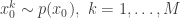
First introduce notation for the “particle cloud”: , , . Initialise the particle filter with , where and (note that is undefined). Now suppose at time we have a sample from : . First resample by sampling , . Here we use for the discrete distribution on with probability mass function . Next sample . Set and . Finally, propagate to the next step… We define the filter’s estimate of likelihood as and . See Doucet et al (2001) for further theoretical background on particle filters and SMC more generally.
Describing the filter carefully as above allows us to write down the joint density of all random variables in the filter as
For PMMH we also sample a final index from giving the joint density
We write the final selected trajectory as
where , and . If we now think about the structure of the PMMH algorithm, our proposal on the space of all random variables in the problem is in fact
and by considering the proposal and the acceptance ratio, it is clear that detailed balance for the chain is satisfied by the target with density proportional to
We want to show that this target marginalises down to the correct posterior when we consider just the parameters and the selected trajectory. But if we consider the terms in the joint distribution of the proposal corresponding to the trajectory selected by , this is given by
which, by expanding the in terms of the unnormalised weights, simplifies to
It is worth dwelling on this result, as this is the key insight required to understand why the PMMH algorithm works. The whole point is that the terms in the joint density of the proposal corresponding to the selected trajectory exactly represent the required joint distribution modulo a couple of normalising constants, one of which is the particle filter’s estimate of marginal likelihood. Thus, by including in the acceptance ratio, we knock out the normalising constant, allowing all of the other terms in the proposal to be marginalised away. In other words, the target of the chain can be written as proportional to
The other terms are all probabilities of random variables which do not occur elsewhere in the target, and hence can all be marginalised away to leave the correct posterior
Thus the PMMH algorithm targets the correct posterior for any number of particles, . Also note the implied uniform distribution on the selected indices in the target.
The pseudo-marginal approach to MCMC for Bayesian inference
In a previous post I described a generalisation of the Metropolis Hastings MCMC algorithm which uses unbiased Monte Carlo estimates of likelihood in the acceptance ratio, but is nevertheless exact, when considered as a pseudo-marginal approach to “exact approximate” MCMC. To be useful in the context of Bayesian inference, we need to be able to compute unbiased estimates of the (marginal) likelihood of the data given some proposed model parameters with any “latent variables” integrated out.
To be more precise, consider a model for data with parameters of the form together with a prior on , , giving a joint model
Suppose now that interest is in the posterior distribution
We can construct a fairly generic (marginal) MCMC scheme for this posterior by first proposing from some fairly arbitrary proposal distribution and then accepting the value with probability where
This method is great provided that the (marginal) likelihood of the data is available to us analytically, but in many (most) interesting models it is not. However, in the previous post I explained why substituting in a Monte Carlo estimate will still lead to the exact posterior if the estimate is unbiased in the sense that . Consequently, sources of (cheap) unbiased Monte Carlo estimates of (marginal) likelihood are of potential interest in the development of exact MCMC algorithms.
Latent variables and marginalisation
Often the reason that we cannot evaluate is that there are latent variables in the problem, and the model for the data is conditional on those latent variables. Explicitly, if we denote the latent variables by , then the joint distribution for the model takes the form
Now since
there is a simple and obvious Monte Carlo strategy for estimating provided that we can evaluate and simulate realisations from . That is, simulate values from for some suitably large , and then put
It is clear by the law of large numbers that this estimate will converge to as . That is, is a consistent estimate of . However, a moment’s thought reveals that this estimate is not only consistent, but also unbiased, since each term in the sum has expectation . This simple Monte Carlo estimate of likelihood can therefore be substituted into a Metropolis-Hastings acceptance ratio without affecting the (marginal) target distribution of the Markov chain. Note that this estimate of marginal likelihood is sometimes referred to as the Rao-Blackwellised estimate, due to its connection with the Rao-Blackwell theorem.
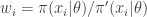
Importance sampling
Suppose now that we cannot sample values directly from , but can sample instead from a distribution having the same support as . We can then instead produce an importance sampling estimate for by noting that
Consequently, samples from can be used to construct the estimate
which again is clearly both consistent and unbiased. This estimate is often written
where . The weights, , are known as importance weights.
Importance resampling
An idea closely related to that of importance sampling is that of importance resampling where importance weights are used to resample a sample in order to equalise the weights, often prior to a further round of weighting and resampling. The basic idea is to generate an approximate sample from a target density using values sampled from an auxiliary distribution , where we now supress any dependence of the distributions on model parameters, .
First generate a sample from and compute weights . Then compute normalised weights . Generate a new sample of size by sampling times with replacement from the original sample with the probability of choosing each value determined by its normalised weight.
As an example, consider using a sample from the Cauchy distribution as an auxiliary distribution for approximately sampling standard normal random quantities. We can do this using a few lines of R as follows.
Note that we don’t actually need to compute the normalised weights, as the sample function will do this for us. Note also that the average weight will be close to one. It should be clear that the expected value of the weights will be exactly 1 when both the target and auxiliary densities are correctly normalised. Also note that the procedure can be used when one or both of the densities are not correctly normalised, since the weights will be normalised prior to sampling anyway. Note that in this case the expected weight will be the (ratio of) normalising constant(s), and so looking at the average weight will give an estimate of the normalising constant.
Note that the importance sampling procedure is approximate. Unlike a technique such as rejection sampling, which leads to samples having exactly the correct distribution, this is not the case here. Indeed, it is clear that in the case, the final sample will be exactly drawn from the auxiliary and not the target. The procedure is asymptotic, in that it improves as the sample size increases, tending to the exact target as .
We can understand why importance resampling works by first considering the univariate case, using correctly normalised densities. Consider a very large number of particles, . The proportion of the auxiliary samples falling in a small interval will be , corresponding to roughly particles. The weight for each of those particles will be , and since the expected weight of a random particle is 1, the sum of all weights will be (roughly) , leading to normalised weights for the particles near of . The combined weight of all particles in is therefore . Clearly then, when we resample times we expect to select roughly particles from this interval. This corresponds to a proportion , corresponding to a density of in the final sample.
Obviously the above argument is very informal, but can be tightened up into a reasonably rigorous proof for the 1d case without too much effort, and the multivariate extension is also reasonably clear.
The bootstrap particle filter
The bootstrap particle filter is an iterative method for carrying out Bayesian inference for dynamic state space (partially observed Markov process) models, sometimes also known as hidden Markov models (HMMs). Here, an unobserved Markov process, governed by a transition kernel is partially observed via some measurement model leading to data . The idea is to make inference for the hidden states given the data . The method is a very simple application of the importance resampling technique. At each time, , we assume that we have a (approximate) sample from and use importance resampling to generate an approximate sample from .
More precisely, the procedure is initialised with a sample from with uniform normalised weights . Then suppose that we have a weighted sample from . First generate an equally weighted sample by resampling with replacement times to obtain (giving an approximate random sample from ). Note that each sample is independently drawn from . Next propagate each particle forward according to the Markov process model by sampling (giving an approximate random sample from ). Then for each of the new particles, compute a weight , and then a normalised weight .
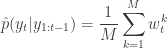
It is clear from our understanding of importance resampling that these weights are appropriate for representing a sample from , and so the particles and weights can be propagated forward to the next time point. It is also clear that the average weight at each time gives an estimate of the marginal likelihood of the current data point given the data so far. So we define
and
Again, from our understanding of importance resampling, it should be reasonably clear that is a consistent estimator of . It is much less clear, but nevertheless true that this estimator is also unbiased. The standard reference for this fact is Del Moral (2004), but this is a rather technical monograph. A much more accessible proof (for a very general particle filter) is given in Pitt et al (2011).
It should therefore be clear that if one is interested in developing MCMC algorithms for state space models, one can use a pseudo-marginal MCMC scheme, substituting in from a bootstrap particle filter in place of . This turns out to be a simple special case of the particle marginal Metropolis-Hastings (PMMH) algorithm described in Andreiu et al (2010). However, the PMMH algorithm in fact has the full joint posterior as its target. I will explain the PMMH algorithm in a subsequent post.
In this post I will try and explain an important idea behind some recent developments in MCMC theory. First, let me give some motivation. Suppose you are trying to implement a Metropolis-Hastings algorithm, as discussed in a previous post (required reading!), but a key likelihood term needed for the acceptance ratio is difficult to evaluate (most likely it is a marginal likelihood of some sort). If it is possible to obtain a Monte-Carlo estimate for that likelihood term (which it sometimes is, for example, using importance sampling), one could obviously just plug it in to the acceptance ratio and hope for the best. What is not at all obvious is that if your Monte-Carlo estimate satisfies some fairly weak property then the equilibrium distribution of the Markov chain will remain exactly as it would be if the exact likelihood had been available. Furthermore, it is exact even if the Monte-Carlo estimate is very noisy and imprecise (though the mixing of the chain will be poorer in this case). This is the “exact approximate” pseudo-marginal MCMC approach. To give credit where it is due, the idea was first introduced by Mark Beaumont in Beaumont (2003), where he was using an importance sampling based approximate likelihood in the context of a statistical genetics example. This was later picked up by Christophe Andrieu and Gareth Roberts, who studied the technical properties of the approach in Andrieu and Roberts (2009). The idea is turning out to be useful in several contexts, and in particular, underpins the interesting new Particle MCMC algorithms of Andrieu et al (2010), which I will discuss in a future post. I’ve heard Mark, Christophe, Gareth and probably others present this concept, but this post is most strongly inspired by a talk that Christophe gave at the IMS 2010 meeting in Gothenburg this summer.
The pseudo-marginal Metropolis-Hastings algorithm
Let’s focus on the simplest version of the problem, where we want to sample from a target using a proposal . As explained previously, the required Metropolis-Hastings acceptance ratio will take the form
Here we are assuming that is difficult to evaluate (usually because it is a marginalised version of some higher-dimensional distribution), but that a Monte-Carlo estimate of , which we shall denote , can be computed. We can obviously just substitute this estimate into the acceptance ratio to get
but it is not immediately clear that in many cases this will lead to the Markov chain having an equilibrium distribution that is exactly. It turns out that it is sufficient that the likelihood estimate, is non-negative, and unbiased, in the sense that , where the expectation is with respect to the Monte-Carlo error for a given fixed value of . In fact, as we shall see, this condition is actually a bit stronger than is really required.
Put , representing the noise in the Monte-Carlo estimate of , and suppose that (note that in an abuse of notation, the function is unrelated to ). The main condition we will assume is that , where is a constant independent of . In the case of , we have the (typical) special case of . For now, we will also assume that , but we will consider relaxing this constraint later.
The key to understanding the pseudo-marginal approach is to realise that at each iteration of the MCMC algorithm a new value of is being proposed in addition to a new value for . If we regard the proposal mechanism as a joint update of and , it is clear that the proposal generates from the density , and we can re-write our “approximate” acceptance ratio as
Inspection of this acceptance ratio reveals that the target of the chain must be (proportional to)
This is a joint density for , but the marginal for can be obtained by integrating over the range of with respect to . Using the fact that , this then clearly gives a density proportional to , and this is precisely the target that we require. Note that for this to work, we must keep the old value of from one iteration to the next – that is, we must keep and re-use our noisy value to include in the acceptance ratio for our next MCMC iteration – we should not compute a new Monte-Carlo estimate for the likelihood of the old state of the chain.
Examples
We will consider again the example from the previous post – simulation of a chain with a N(0,1) target using uniform innovations. Using R, the main MCMC loop takes the form
pmmcmc<-function(n=1000,alpha=0.5)
{
        vec=vector("numeric", n)
        x=0
        oldlik=noisydnorm(x)
        vec[1]=x
        for (i in 2:n) {
                innov=runif(1,-alpha,alpha)
                can=x+innov
                lik=noisydnorm(can)
                aprob=lik/oldlik
                u=runif(1)
                if (u < aprob) {
                        x=can
                        oldlik=lik
			}
                vec[i]=x
        }
        vec
}
Here we are assuming that we are unable to compute dnorm exactly, but instead only a Monte-Carlo estimate called noisydnorm. We can start with the following implementation
noisydnorm<-function(z)
{
	dnorm(z)*rexp(1,1)
}
Each time this function is called, it will return a non-negative random quantity whose expectation is dnorm(z). We can now run this code as follows.
So we see that we have exactly the right N(0,1) target, despite using the (very) noisy noisydnorm function in place of the dnorm function. This noisy likelihood function is clearly unbiased. However, as already discussed, a constant bias in the noise is also acceptable, as the following function shows.
noisydnorm<-function(z)
{
	dnorm(z)*rexp(1,2)
}
Re-running the code with this function also leads to the correct equilibrium distribution for the chain. However, it really does matter that the bias is independent of the state of the chain, as the following function shows.
Running with this function leads to the wrong equilibrium. However, it is OK for the distribution of the noise to depend on the state, as long as its expectation does not. The following function illustrates this.
This works just fine. So far we have been assuming that our noisy likelihood estimates are non-negative. This is clearly desirable, as otherwise we could wind up with negative Metropolis-Hasting ratios. However, as long as we are careful about exactly what we mean, even this non-negativity condition may be relaxed. The following function illustrates the point.
noisydnorm<-function(z)
{
	dnorm(z)*rnorm(1,1)
}
Despite the fact that this function will often produce negative values, the equilibrium distribution of the chain still seems to be correct! An even more spectacular example follows.
noisydnorm<-function(z)
{
	dnorm(z)*rnorm(1,0)
}
Astonishingly, this one works too, despite having an expected value of zero! However, the following doesn’t work, even though it too has a constant expectation of zero.
I don’t have time to explain exactly what is going on here, so the precise details are left as an exercise for the reader. Suffice to say that the key requirement is that it is the distribution of W conditioned to be non-negative which must have the constant bias property – something clearly violated by the final noisydnorm example.
Before finishing this post, it is worth re-emphasising the issue of re-using old Monte-Carlo estimates. The following function will not work (exactly), though in the case of good Monte-Carlo estimates will often work tolerably well.
approxmcmc<-function(n=1000,alpha=0.5)
{
        vec=vector("numeric", n)
        x=0
        vec[1]=x
        for (i in 2:n) {
                innov=runif(1,-alpha,alpha)
                can=x+innov
                lik=noisydnorm(can)
                oldlik=noisydnorm(x)
                aprob=lik/oldlik
                u=runif(1)
                if (u < aprob) {
                        x=can
			}
                vec[i]=x
        }
        vec
}
In a subsequent post I will show how these ideas can be put into practice in the context of a Bayesian inference example.


 random quantities to construct a Monte Carlo estimate of the integral
 .
. separate computations, and use a map to compute the required Monte Carlo sums.
 , latent variables
  and data
  , of the form
 . On the other hand, the PMMH algorithm is an MCMC algorithm which targets the full joint posterior distribution
  . Now, the PMMH scheme does reduce to the pseudo-marginal scheme if samples of
  ). Below I will describe the algorithm and explain why it works, but first it is necessary to understand the relationship between marginal, joint and “likelihood-free” MCMC updating schemes for such latent variable models.
 is proposed from
  and accepted with probability
  , where
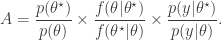
 required in the acceptance ratio is often difficult to compute.
 even when we can’t evaluate it, or marginalise
  is simulated from the model
  . The pair
  is then jointly accepted with ratio
 . The pair
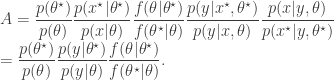
 , as the algorithms above. First, a proposed new
  is generated by running a bootstrap particle filter (as described in the previous post, and below) using the proposed new model parameters,
  is accepted using the Metropolis-Hastings ratio
 is the particle filter’s (unbiased) estimate of marginal likelihood, described in the previous post, and below. Note that this approach tends to the perfect joint/marginal updating scheme as the number of particles used in the filter tends to infinity. Note also that for a single particle, the particle filter just blindly forward simulates from
  and that the filter’s estimate of marginal likelihood is just the observed data likelihood
  leading precisely to the simple likelihood-free scheme. To understand for an arbitrary finite number of particles,
  , one needs to think carefully about the structure of the particle filter.
 ,
,  ,
,  . Initialise the particle filter with
  , where
  and
and  (note that
  is undefined). Now suppose at time
  we have a sample from
  :
:  . First resample by sampling
  ,
,  . Here we use
  for the discrete distribution on
  with probability mass function
  . Next sample
  . Set
. Set 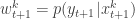 and
and 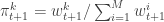 . Finally, propagate
  to the next step… We define the filter’s estimate of likelihood as
 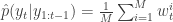 and
and 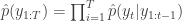 . See
. See ![\displaystyle \tilde{q}(\mathbf{x}_0,\ldots,\mathbf{x}_T,\mathbf{a}_0,\ldots,\mathbf{a}_{T-1}) = \left[\prod_{k=1}^M p(x_0^k)\right] \left[\prod_{t=0}^{T-1} \prod_{k=1}^M \pi_t^{a_t^k} p(x_{t+1}^k|x_t^{a_t^k}) \right]](https://s0.wp.com/latex.php?latex=%5Cdisplaystyle++%5Ctilde%7Bq%7D%28%5Cmathbf%7Bx%7D_0%2C%5Cldots%2C%5Cmathbf%7Bx%7D_T%2C%5Cmathbf%7Ba%7D_0%2C%5Cldots%2C%5Cmathbf%7Ba%7D_%7BT-1%7D%29++%3D+%5Cleft%5B%5Cprod_%7Bk%3D1%7D%5EM+p%28x_0%5Ek%29%5Cright%5D+%5Cleft%5B%5Cprod_%7Bt%3D0%7D%5E%7BT-1%7D++++%5Cprod_%7Bk%3D1%7D%5EM+%5Cpi_t%5E%7Ba_t%5Ek%7D+p%28x_%7Bt%2B1%7D%5Ek%7Cx_t%5E%7Ba_t%5Ek%7D%29+%5Cright%5D++&bg=ffffff&fg=333333&s=0&c=20201002)
 from
from  giving the joint density

 , and
, and  . If we now think about the structure of the PMMH algorithm, our proposal on the space of all random variables in the problem is in fact

 when we consider just the parameters and the selected trajectory. But if we consider the terms in the joint distribution of the proposal corresponding to the trajectory selected by
 ![\displaystyle p_\theta(x_0^{b_0^{k'}})\left[\prod_{t=0}^{T-1} \pi_t^{b_t^{k'}} p_\theta(x_{t+1}^{b_{t+1}^{k'}}|x_t^{b_t^{k'}})\right]\pi_T^{k'} = p_\theta(x_{0:T}^{k'})\prod_{t=0}^T \pi_t^{b_t^{k'}}](https://s0.wp.com/latex.php?latex=%5Cdisplaystyle++p_%5Ctheta%28x_0%5E%7Bb_0%5E%7Bk%27%7D%7D%29%5Cleft%5B%5Cprod_%7Bt%3D0%7D%5E%7BT-1%7D+%5Cpi_t%5E%7Bb_t%5E%7Bk%27%7D%7D++++p_%5Ctheta%28x_%7Bt%2B1%7D%5E%7Bb_%7Bt%2B1%7D%5E%7Bk%27%7D%7D%7Cx_t%5E%7Bb_t%5E%7Bk%27%7D%7D%29%5Cright%5D%5Cpi_T%5E%7Bk%27%7D++%3D++p_%5Ctheta%28x_%7B0%3AT%7D%5E%7Bk%27%7D%29%5Cprod_%7Bt%3D0%7D%5ET+%5Cpi_t%5E%7Bb_t%5E%7Bk%27%7D%7D++&bg=ffffff&fg=333333&s=0&c=20201002)
 in terms of the unnormalised weights, simplifies to
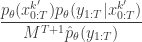
 in the acceptance ratio, we knock out the normalising constant, allowing all of the other terms in the proposal to be marginalised away. In other words, the target of the chain can be written as proportional to

 together with a prior on
  , giving a joint model

 from some fairly arbitrary proposal distribution and then accepting the value with probability
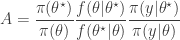
 will still lead to the exact posterior if the estimate is unbiased in the sense that
 ![E[\hat\pi(y|\theta)]=\pi(y|\theta)](https://s0.wp.com/latex.php?latex=E%5B%5Chat%5Cpi%28y%7C%5Ctheta%29%5D%3D%5Cpi%28y%7C%5Ctheta%29&bg=ffffff&fg=333333&s=0&c=20201002) . Consequently, sources of (cheap) unbiased Monte Carlo estimates of (marginal) likelihood are of potential interest in the development of exact MCMC algorithms.
. Consequently, sources of (cheap) unbiased Monte Carlo estimates of (marginal) likelihood are of potential interest in the development of exact MCMC algorithms.

 and simulate realisations from
  . That is, simulate values
  from
from  , and then put
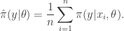
 . That is,
  having the same support as


 . The weights,
  , are known as importance weights.
 using values sampled from an auxiliary distribution
  , where we now supress any dependence of the distributions on model parameters,
  from
from  . Then compute normalised weights
 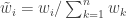 . Generate a new sample of size
  case, the final sample will be exactly drawn from the auxiliary and not the target. The procedure is asymptotic, in that it improves as the sample size increases, tending to the exact target as
  . The proportion of the auxiliary samples falling in a small interval
  will be
  , corresponding to roughly
  particles. The weight for each of those particles will be
  , and since the expected weight of a random particle is 1, the sum of all weights will be (roughly)
 ![\tilde{w}(x)=\pi(x)/[N\pi'(x)]](https://s0.wp.com/latex.php?latex=%5Ctilde%7Bw%7D%28x%29%3D%5Cpi%28x%29%2F%5BN%5Cpi%27%28x%29%5D&bg=ffffff&fg=333333&s=0&c=20201002) . The combined weight of all particles in
. The combined weight of all particles in  . Clearly then, when we resample
  particles from this interval. This corresponds to a proportion
  , corresponding to a density of
  governed by a transition kernel
  is partially observed via some measurement model
  leading to data
  . The idea is to make inference for the hidden states
  . The method is a very simple application of the importance resampling technique. At each time,
  .
. with uniform normalised weights
  . Then suppose that we have a weighted sample
  from
from 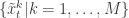 (giving an approximate random sample from
  . Next propagate each particle forward according to the Markov process model by sampling
  (giving an approximate random sample from
  ). Then for each of the new particles, compute a weight
  .
. 

 is a consistent estimator of
  . It is much less clear, but nevertheless true that this estimator is also unbiased. The standard reference for this fact is
  . This turns out to be a simple special case of the particle marginal Metropolis-Hastings (PMMH) algorithm described in
  using a proposal
  . As explained previously, the required Metropolis-Hastings acceptance ratio will take the form
 , can be computed. We can obviously just substitute this estimate into the acceptance ratio to get
 , where the expectation is with respect to the Monte-Carlo error for a given fixed value of
  , representing the noise in the Monte-Carlo estimate of
  (note that in an abuse of notation, the function
  is unrelated to
  , where
  is a constant independent of
  , we have the (typical) special case of
  , but we will consider relaxing this constraint later.
  is being proposed in addition to a new value for
  , it is clear that the proposal generates
  from the density
 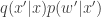 , and we can re-write our “approximate” acceptance ratio as
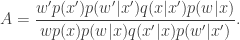

 , but the marginal for
