Introduction
In the previous post I showed how to write your own general-purpose monadic probabilistic programming language from scratch in 50 lines of (Scala) code. That post is a pre-requisite for this one, so if you haven’t read it, go back and have a quick skim through it before proceeding. In that post I tried to keep everything as simple as possible, but at the expense of both elegance and efficiency. In this post I’ll address one problem with the implementation from that post – the memory (and computational) overhead associated with forming the Cartesian product of particle sets during monadic binding (flatMap). So if particle sets are typically of size 

Materials for this post can be found in my blog repo, and a draft of this post itself can be found in the form of an executable tut document.
An SMC-based monad
The idea behind the approach to binding used in this monad is to mimic the “predict” step of a bootstrap particle filter. Here, for each particle in the source distribution, exactly one particle is drawn from the required conditional distribution and paired with the source particle, preserving the source particle’s original weight. So, in order to operationalise this, we will need a draw method adding into our probability monad. It will also simplify things to add a flatMap method to our Particle type constructor.
To follow along, you can type sbt console from the min-ppl2 directory of my blog repo, then paste blocks of code one at a time.
  import breeze.stats.{distributions => bdist}
  import breeze.linalg.DenseVector
  import cats._
  import cats.implicits._

  implicit val numParticles = 2000

  case class Particle[T](v: T, lw: Double) { // value and log-weight
    def map[S](f: T => S): Particle[S] = Particle(f(v), lw)
    def flatMap[S](f: T => Particle[S]): Particle[S] = {
      val ps = f(v)
      Particle(ps.v, lw + ps.lw)
    }
  }
I’ve added a dependence on cats here, so that we can use some derived methods, later. To take advantage of this, we must provide evidence that our custom types conform to standard type class interfaces. For example, we can provide evidence that Particle[_] is a monad as follows.
  implicit val particleMonad = new Monad[Particle] {
    def pure[T](t: T): Particle[T] = Particle(t, 0.0)
    def flatMap[T,S](pt: Particle[T])(f: T => Particle[S]): Particle[S] = pt.flatMap(f)
    def tailRecM[T,S](t: T)(f: T => Particle[Either[T,S]]): Particle[S] = ???
  }
The technical details are not important for this post, but we’ll see later what this can give us.
We can now define our Prob[_] monad in the following way.
  trait Prob[T] {
    val particles: Vector[Particle[T]]
    def draw: Particle[T]
    def mapP[S](f: T => Particle[S]): Prob[S] = Empirical(particles map (_ flatMap f))
    def map[S](f: T => S): Prob[S] = mapP(v => Particle(f(v), 0.0))
    def flatMap[S](f: T => Prob[S]): Prob[S] = mapP(f(_).draw)
    def resample(implicit N: Int): Prob[T] = {
      val lw = particles map (_.lw)
      val mx = lw reduce (math.max(_,_))
      val rw = lw map (lwi => math.exp(lwi - mx))
      val law = mx + math.log(rw.sum/(rw.length))
      val ind = bdist.Multinomial(DenseVector(rw.toArray)).sample(N)
      val newParticles = ind map (i => particles(i))
      Empirical(newParticles.toVector map (pi => Particle(pi.v, law)))
    }
    def cond(ll: T => Double): Prob[T] = mapP(v => Particle(v, ll(v)))
    def empirical: Vector[T] = resample.particles.map(_.v)
  }

  case class Empirical[T](particles: Vector[Particle[T]]) extends Prob[T] {
    def draw: Particle[T] = {
      val lw = particles map (_.lw)
      val mx = lw reduce (math.max(_,_))
      val rw = lw map (lwi => math.exp(lwi - mx))
      val law = mx + math.log(rw.sum/(rw.length))
      val idx = bdist.Multinomial(DenseVector(rw.toArray)).draw
      Particle(particles(idx).v, law)
    }
  }
As before, if you are pasting code blocks into the REPL, you will need to use :paste mode to paste these two definitions together.
The essential structure is similar to that from the previous post, but with a few notable differences. Most fundamentally, we now require any concrete implementation to provide a draw method returning a single particle from the distribution. Like before, we are not worrying about purity of functional code here, and using a standard random number generator with a globally mutating state. We can define a mapP method (for “map particle”) using the new flatMap method on Particle, and then use that to define map and flatMap for Prob[_]. Crucially, draw is used to define flatMap without requiring a Cartesian product of distributions to be formed.
We add a draw method to our Empirical[_] implementation. This method is computationally intensive, so it will still be computationally problematic to chain several flatMaps together, but this will no longer be flatMaps. There is obviously some code duplication between the draw method on Empirical and the resample method on Prob, but I’m not sure it’s worth factoring out.
It is worth noting that neither flatMap nor cond triggers resampling, so the user of the library is now responsible for resampling when appropriate.
We can provide evidence that Prob[_] forms a monad just like we did Particle[_].
  implicit val probMonad = new Monad[Prob] {
    def pure[T](t: T): Prob[T] = Empirical(Vector(Particle(t, 0.0)))
    def flatMap[T,S](pt: Prob[T])(f: T => Prob[S]): Prob[S] = pt.flatMap(f)
    def tailRecM[T,S](t: T)(f: T => Prob[Either[T,S]]): Prob[S] = ???
  }
Again, we’ll want to be able to create a distribution from an unweighted collection of values.
  def unweighted[T](ts: Vector[T], lw: Double = 0.0): Prob[T] =
    Empirical(ts map (Particle(_, lw)))
We will again define an implementation for distributions with tractable likelihoods, which are therefore easy to condition on. They will typically also be easy to draw from efficiently, and we will use this fact, too.
  trait Dist[T] extends Prob[T] {
    def ll(obs: T): Double
    def ll(obs: Seq[T]): Double = obs map (ll) reduce (_+_)
    def fit(obs: Seq[T]): Prob[T] = mapP(v => Particle(v, ll(obs)))
    def fitQ(obs: Seq[T]): Prob[T] = Empirical(Vector(Particle(obs.head, ll(obs))))
    def fit(obs: T): Prob[T] = fit(List(obs))
    def fitQ(obs: T): Prob[T] = fitQ(List(obs))
  }
We can give implementations of this for a few standard distributions.
  case class Normal(mu: Double, v: Double)(implicit N: Int) extends Dist[Double] {
    lazy val particles = unweighted(bdist.Gaussian(mu, math.sqrt(v)).
      sample(N).toVector).particles
    def draw = Particle(bdist.Gaussian(mu, math.sqrt(v)).draw, 0.0)
    def ll(obs: Double) = bdist.Gaussian(mu, math.sqrt(v)).logPdf(obs)
  }

  case class Gamma(a: Double, b: Double)(implicit N: Int) extends Dist[Double] {
    lazy val particles = unweighted(bdist.Gamma(a, 1.0/b).
      sample(N).toVector).particles
    def draw = Particle(bdist.Gamma(a, 1.0/b).draw, 0.0)
    def ll(obs: Double) = bdist.Gamma(a, 1.0/b).logPdf(obs)
  }

  case class Poisson(mu: Double)(implicit N: Int) extends Dist[Int] {
    lazy val particles = unweighted(bdist.Poisson(mu).
      sample(N).toVector).particles
    def draw = Particle(bdist.Poisson(mu).draw, 0.0)
    def ll(obs: Int) = bdist.Poisson(mu).logProbabilityOf(obs)
  }
Note that we now have to provide an (efficient) draw method for each implementation, returning a single draw from the distribution as a Particle with a (raw) weight of 1 (log weight of 0).
We are done. It’s a few more lines of code than that from the previous post, but this is now much closer to something that could be used in practice to solve actual inference problems using a reasonable number of particles. But to do so we will need to be careful do avoid deep monadic binding. This is easiest to explain with a concrete example.
Using the SMC-based probability monad in practice
Monadic binding and applicative structure
As explained in the previous post, using Scala’s for-expressions for monadic binding gives a natural and elegant PPL for our probability monad “for free”. This is fine, and in general there is no reason why using it should lead to inefficient code. However, for this particular probability monad implementation, it turns out that deep monadic binding comes with a huge performance penalty. For a concrete example, consider the following specification, perhaps of a prior distribution over some independent parameters.
    val prior = for {
      x <- Normal(0,1)
      y <- Gamma(1,1)
      z <- Poisson(10)
    } yield (x,y,z)
Don’t paste that into the REPL – it will take an age to complete!
Again, I must emphasise that there is nothing wrong with this specification, and there is no reason in principle why such a specification can’t be computationally efficient – it’s just a problem for our particular probability monad. We can begin to understand the problem by thinking about how this will be de-sugared by the compiler. Roughly speaking, the above will de-sugar to the following nested flatMaps.
    val prior2 =
      Normal(0,1) flatMap {x =>
        Gamma(1,1) flatMap {y =>
          Poisson(10) map {z =>
            (x,y,z)}}}
Again, beware of pasting this into the REPL.
So, although written from top to bottom, the nesting is such that the flatMaps collapse from the bottom-up. The second flatMap (the first to collapse) isn’t such a problem here, as the Poisson has a 
draw method. But the result is an empirical distribution, which has an 
flatMap (the second to collapse) is an 
flatMaps will be exponential in the number of monadic binds. So, looking back at the for expression, the problem is that there are three <-. The last one isn’t a problem since it corresponds to a map, and the second last one isn’t a problem, since the final distribution is tractable with an draw method. The problem is the first <-, corresponding to a flatMap of one empirical distribution with respect to another. For our particular probability monad, it’s best to avoid these if possible.
The interesting thing to note here is that because the distributions are independent, there is no need for them to be sequenced. They could be defined in any order. In this case it makes sense to use the applicative structure implied by the monad.
Now, since we have told cats that Prob[_] is a monad, it can provide appropriate applicative methods for us automatically. In Cats, every monad is assumed to be also an applicative functor (which is true in Cartesian closed categories, and Cats implicitly assumes that all functors and monads are defined over CCCs). So we can give an alternative specification of the above prior using applicative composition.
 val prior3 = Applicative[Prob].tuple3(Normal(0,1), Gamma(1,1), Poisson(10))
// prior3: Wrapped.Prob[(Double, Double, Int)] = Empirical(Vector(Particle((-0.057088546468105204,0.03027578552505779,9),0.0), Particle((-0.43686658266043743,0.632210127012762,14),0.0), Particle((-0.8805715148936012,3.4799656228544706,4),0.0), Particle((-0.4371726407147289,0.0010707859994652403,12),0.0), Particle((2.0283297088320755,1.040984491158822,10),0.0), Particle((1.2971862986495886,0.189166705596747,14),0.0), Particle((-1.3111333817551083,0.01962422606642761,9),0.0), Particle((1.6573851896142737,2.4021836368401415,9),0.0), Particle((-0.909927220984726,0.019595551644771683,11),0.0), Particle((0.33888133893822464,0.2659823344145805,10),0.0), Particle((-0.3300797295729375,3.2714740256437667,10),0.0), Particle((-1.8520554352884224,0.6175322756460341,10),0.0), Particle((0.541156780497547...
This one is mathematically equivalent, but safe to paste into your REPL, as it does not involve deep monadic binding, and can be used whenever we want to compose together independent components of a probabilistic program. Note that “tupling” is not the only possibility – Cats provides a range of functions for manipulating applicative values.
This is one way to avoid deep monadic binding, but another strategy is to just break up a large for expression into separate smaller for expressions. We can examine this strategy in the context of state-space modelling.
Particle filtering for a non-linear state-space model
We can now re-visit the DGLM example from the previous post. We began by declaring some observations and a prior.
    val data = List(2,1,0,2,3,4,5,4,3,2,1)
// data: List[Int] = List(2, 1, 0, 2, 3, 4, 5, 4, 3, 2, 1)

    val prior = for {
      w <- Gamma(1, 1)
      state0 <- Normal(0.0, 2.0)
    } yield (w, List(state0))
// prior: Wrapped.Prob[(Double, List[Double])] = Empirical(Vector(Particle((4.220683377724395,List(0.37256749723762683)),0.0), Particle((0.4436668049925418,List(-1.0053578391265572)),0.0), Particle((0.9868899648436931,List(-0.6985099310193449)),0.0), Particle((0.13474375773634908,List(0.9099291736792412)),0.0), Particle((1.9654021747685184,List(-0.042127103727998175)),0.0), Particle((0.21761202474220223,List(1.1074616830012525)),0.0), Particle((0.31037163527711015,List(0.9261849914020324)),0.0), Particle((1.672438830781466,List(0.01678529855289384)),0.0), Particle((0.2257151759143097,List(2.5511304854128354)),0.0), Particle((0.3046489890769499,List(3.2918304533361398)),0.0), Particle((1.5115941814057159,List(-1.633612165168878)),0.0), Particle((1.4185906813831506,List(-0.8460922678989864))...
Looking carefully at the for-expression, there are just two <-, and the distribution on the RHS of the flatMap is tractable, so this is just
Next, let’s look at the function to add a time point, which previously looked something like the following.
    def addTimePointSIS(current: Prob[(Double, List[Double])],
      obs: Int): Prob[(Double, List[Double])] = {
      println(s"Conditioning on observation: $obs")
      for {
        tup <- current
        (w, states) = tup
        os = states.head
        ns <- Normal(os, w)
        _ <- Poisson(math.exp(ns)).fitQ(obs)
      } yield (w, ns :: states)
    }
// addTimePointSIS: (current: Wrapped.Prob[(Double, List[Double])], obs: Int)Wrapped.Prob[(Double, List[Double])]
Recall that our new probability monad does not automatically trigger resampling, so applying this function in a fold will lead to a simple sampling importance sampling (SIS) particle filter. Typically, the bootstrap particle filter includes resampling after each time point, giving a special case of a sampling importance resampling (SIR) particle filter, which we could instead write as follows.
    def addTimePointSimple(current: Prob[(Double, List[Double])],
      obs: Int): Prob[(Double, List[Double])] = {
      println(s"Conditioning on observation: $obs")
      val updated = for {
        tup <- current
        (w, states) = tup
        os = states.head
        ns <- Normal(os, w)
        _ <- Poisson(math.exp(ns)).fitQ(obs)
      } yield (w, ns :: states)
      updated.resample
    }
// addTimePointSimple: (current: Wrapped.Prob[(Double, List[Double])], obs: Int)Wrapped.Prob[(Double, List[Double])]
This works fine, but we can see that there are three <- in this for expression. This leads to a flatMap with an empirical distribution on the RHS, and hence is
    def addTimePoint(current: Prob[(Double, List[Double])],
      obs: Int): Prob[(Double, List[Double])] = {
      println(s"Conditioning on observation: $obs")
      val predict = for {
        tup <- current
        (w, states) = tup
        os = states.head
        ns <- Normal(os, w)
      }
      yield (w, ns :: states)
      val updated = for {
        tup <- predict
        (w, states) = tup
        st = states.head
        _ <- Poisson(math.exp(st)).fitQ(obs)
      } yield (w, states)
      updated.resample
    }
// addTimePoint: (current: Wrapped.Prob[(Double, List[Double])], obs: Int)Wrapped.Prob[(Double, List[Double])]
By breaking the for expression into two: the first for the “predict” step and the second for the “update” (conditioning on the observation), we get two
  import breeze.stats.{meanAndVariance => meanVar}
// import breeze.stats.{meanAndVariance=>meanVar}

  val mod = data.foldLeft(prior)(addTimePoint(_,_)).empirical
// Conditioning on observation: 2
// Conditioning on observation: 1
// Conditioning on observation: 0
// Conditioning on observation: 2
// Conditioning on observation: 3
// Conditioning on observation: 4
// Conditioning on observation: 5
// Conditioning on observation: 4
// Conditioning on observation: 3
// Conditioning on observation: 2
// Conditioning on observation: 1
// mod: Vector[(Double, List[Double])] = Vector((0.24822528144246606,List(0.06290285371838457, 0.01633338109272575, 0.8997103339551227, 1.5058726341571411, 1.0579925693609091, 1.1616536515200064, 0.48325623593870665, 0.8457351097543767, -0.1988290999293708, -0.4787511341321954, -0.23212497417019512, -0.15327432440577277)), (1.111430233331792,List(0.6709342824443849, 0.009092797044165657, -0.13203367846117453, 0.4599952735399485, 1.3779288637042504, 0.6176597963402879, 0.6680455419800753, 0.48289163013446945, -0.5994001698510807, 0.4860969602653898, 0.10291798193078927, 1.2878325765987266)), (0.6118925941009055,List(0.6421161986636132, 0.679470360928868, 1.0552459559203342, 1.200835166087372, 1.3690372269589233, 1.8036766847282912, 0.6229883551656629, 0.14872642198313774, -0.122700856878725...

  meanVar(mod map (_._1)) // w
// res0: breeze.stats.meanAndVariance.MeanAndVariance = MeanAndVariance(0.2839184023932576,0.07391602428256917,2000)

  meanVar(mod map (_._2.reverse.head)) // initial state
// res1: breeze.stats.meanAndVariance.MeanAndVariance = MeanAndVariance(0.26057368528422714,0.4802810202354611,2000)

  meanVar(mod map (_._2.head)) // final state
// res2: breeze.stats.meanAndVariance.MeanAndVariance = MeanAndVariance(0.5448036669181697,0.28293080584600894,2000)
Summary and conclusions
Here we have just done some minor tidying up of the rather naive probability monad from the previous post to produce an SMC-based probability monad with improved performance characteristics. Again, we get an embedded probabilistic programming language “for free”. Although the language itself is very flexible, allowing us to construct more-or-less arbitrary probabilistic programs for Bayesian inference problems, we saw that a bug/feature of this particular inference algorithm is that care must be taken to avoid deep monadic binding if reasonable performance is to be obtained. In most cases this is simple to achieve by using applicative composition or by breaking up large for expressions.
There are still many issues and inefficiencies associated with this PPL. In particular, if the main intended application is to state-space models, it would make more sense to tailor the algorithms and implementations to exactly that case. OTOH, if the main concern is a generic PPL, then it would make sense to make the PPL independent of the particular inference algorithm. These are both potential topics for future posts.
Software
- min-ppl2 – code associated with this blog post
- Rainier – a more efficient PPL with similar syntax
- monad-bayes – a Haskell library exploring related ideas

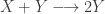

 representing the prey species and
  the predator. I showed how to simulate realisations from this process using the Scala library in the
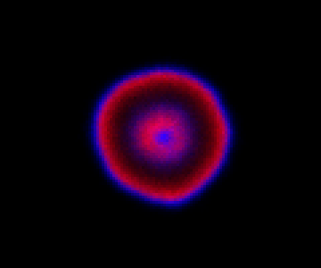

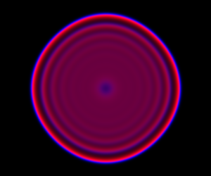


 , red
, red  and blue
  . In this simulation,


 matrix. The idea of variable selection is that probably not all of the p covariates are useful for predicting y, and therefore it would be useful to identify the variables which are, and just use those. Clearly each combination of variables corresponds to a different model, and so the variable selection amounts to choosing among the
  possible models. For large values of p it won’t be practical to consider each possible model separately, and so the idea of Bayesian variable selection is to consider a model containing all of the possible model combinations as sub-models, and the variable selection problem as just another aspect of the model which must be estimated from data. I’m simplifying and glossing over lots of details here, but there is a very nice review paper by
  for each covariate, and introduce these into the model in order to “zero out” inactive covariates. That is we write the ith regression coefficient
  as
as  , so that
  is the regression coefficient when
  , and “doesn’t matter” when
  . There are various ways to choose the prior over
 and
and  of the form
 , latent variables
  and data
  , of the form
 . On the other hand, the PMMH algorithm is an MCMC algorithm which targets the full joint posterior distribution
  . Now, the PMMH scheme does reduce to the pseudo-marginal scheme if samples of
  ). Below I will describe the algorithm and explain why it works, but first it is necessary to understand the relationship between marginal, joint and “likelihood-free” MCMC updating schemes for such latent variable models.
 is proposed from
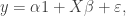
  and accepted with probability
  , where
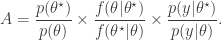
 required in the acceptance ratio is often difficult to compute.
 even when we can’t evaluate it, or marginalise
  is simulated from the model
  . The pair
  is then jointly accepted with ratio
 . The pair
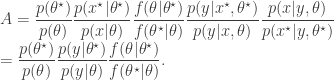
 , as the algorithms above. First, a proposed new
  is generated by running a bootstrap particle filter (as described in the previous post, and below) using the proposed new model parameters,
  is accepted using the Metropolis-Hastings ratio
 is the particle filter’s (unbiased) estimate of marginal likelihood, described in the previous post, and below. Note that this approach tends to the perfect joint/marginal updating scheme as the number of particles used in the filter tends to infinity. Note also that for a single particle, the particle filter just blindly forward simulates from
  and that the filter’s estimate of marginal likelihood is just the observed data likelihood
  leading precisely to the simple likelihood-free scheme. To understand for an arbitrary finite number of particles,
  , one needs to think carefully about the structure of the particle filter.
 ,
,  ,
,  . Initialise the particle filter with
  , where
  and
and  (note that
  is undefined). Now suppose at time
  we have a sample from
  :
:  . First resample by sampling
  ,
,  . Here we use
  for the discrete distribution on
  with probability mass function
  . Next sample
  . Set
. Set 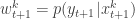 and
and 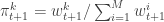 . Finally, propagate
  to the next step… We define the filter’s estimate of likelihood as
 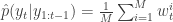 and
and 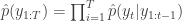 . See
. See ![\displaystyle \tilde{q}(\mathbf{x}_0,\ldots,\mathbf{x}_T,\mathbf{a}_0,\ldots,\mathbf{a}_{T-1}) = \left[\prod_{k=1}^M p(x_0^k)\right] \left[\prod_{t=0}^{T-1} \prod_{k=1}^M \pi_t^{a_t^k} p(x_{t+1}^k|x_t^{a_t^k}) \right]](https://s0.wp.com/latex.php?latex=%5Cdisplaystyle++%5Ctilde%7Bq%7D%28%5Cmathbf%7Bx%7D_0%2C%5Cldots%2C%5Cmathbf%7Bx%7D_T%2C%5Cmathbf%7Ba%7D_0%2C%5Cldots%2C%5Cmathbf%7Ba%7D_%7BT-1%7D%29++%3D+%5Cleft%5B%5Cprod_%7Bk%3D1%7D%5EM+p%28x_0%5Ek%29%5Cright%5D+%5Cleft%5B%5Cprod_%7Bt%3D0%7D%5E%7BT-1%7D++++%5Cprod_%7Bk%3D1%7D%5EM+%5Cpi_t%5E%7Ba_t%5Ek%7D+p%28x_%7Bt%2B1%7D%5Ek%7Cx_t%5E%7Ba_t%5Ek%7D%29+%5Cright%5D++&bg=ffffff&fg=333333&s=0&c=20201002)
 from
from  giving the joint density

 , and
, and  . If we now think about the structure of the PMMH algorithm, our proposal on the space of all random variables in the problem is in fact

 when we consider just the parameters and the selected trajectory. But if we consider the terms in the joint distribution of the proposal corresponding to the trajectory selected by
 ![\displaystyle p_\theta(x_0^{b_0^{k'}})\left[\prod_{t=0}^{T-1} \pi_t^{b_t^{k'}} p_\theta(x_{t+1}^{b_{t+1}^{k'}}|x_t^{b_t^{k'}})\right]\pi_T^{k'} = p_\theta(x_{0:T}^{k'})\prod_{t=0}^T \pi_t^{b_t^{k'}}](https://s0.wp.com/latex.php?latex=%5Cdisplaystyle++p_%5Ctheta%28x_0%5E%7Bb_0%5E%7Bk%27%7D%7D%29%5Cleft%5B%5Cprod_%7Bt%3D0%7D%5E%7BT-1%7D+%5Cpi_t%5E%7Bb_t%5E%7Bk%27%7D%7D++++p_%5Ctheta%28x_%7Bt%2B1%7D%5E%7Bb_%7Bt%2B1%7D%5E%7Bk%27%7D%7D%7Cx_t%5E%7Bb_t%5E%7Bk%27%7D%7D%29%5Cright%5D%5Cpi_T%5E%7Bk%27%7D++%3D++p_%5Ctheta%28x_%7B0%3AT%7D%5E%7Bk%27%7D%29%5Cprod_%7Bt%3D0%7D%5ET+%5Cpi_t%5E%7Bb_t%5E%7Bk%27%7D%7D++&bg=ffffff&fg=333333&s=0&c=20201002)
 in terms of the unnormalised weights, simplifies to
 in the acceptance ratio, we knock out the normalising constant, allowing all of the other terms in the proposal to be marginalised away. In other words, the target of the chain can be written as proportional to

