Part 4: Gradients and the Langevin algorithm
Introduction
This is the fourth part in a series of posts on MCMC-based Bayesian inference for a logistic regression model. If you are new to this series, please go back to Part 1.
In the previous post we saw how the Metropolis algorithm could be used to generate a Markov chain targeting our posterior distribution. In high dimensions the diffusive nature of the Metropolis random walk proposal becomes increasingly inefficient. It is therefore natural to try and develop algorithms that use additional information about the target distribution. In the case of a differentiable log posterior target, a natural first step in this direction is to try and make use of gradient information.
Gradient of a logistic regression model
There are various ways to derive the gradient of our logistic regression model, but it might be simplest to start from the first form of the log likelihood that we deduced in Part 2:
![\displaystyle l(\beta;y) = y^\textsf{T}X\beta - \mathbf{1}^\textsf{T}\log(\mathbf{1}+\exp[X\beta])](https://s0.wp.com/latex.php?latex=%5Cdisplaystyle+l%28%5Cbeta%3By%29+%3D+y%5E%5Ctextsf%7BT%7DX%5Cbeta+-+%5Cmathbf%7B1%7D%5E%5Ctextsf%7BT%7D%5Clog%28%5Cmathbf%7B1%7D%2B%5Cexp%5BX%5Cbeta%5D%29+&bg=ffffff&fg=333333&s=0&c=20201002)
We can write this out in component form as
![\displaystyle l(\beta;y) = \sum_j\sum_j y_iX_{ij}\beta_j - \sum_i\log\left(1+\exp\left[\sum_jX_{ij}\beta_j\right]\right).](https://s0.wp.com/latex.php?latex=%5Cdisplaystyle+l%28%5Cbeta%3By%29+%3D+%5Csum_j%5Csum_j+y_iX_%7Bij%7D%5Cbeta_j+-+%5Csum_i%5Clog%5Cleft%281%2B%5Cexp%5Cleft%5B%5Csum_jX_%7Bij%7D%5Cbeta_j%5Cright%5D%5Cright%29.+&bg=ffffff&fg=333333&s=0&c=20201002)
Differentiating wrt 
![\displaystyle \frac{\partial l}{\partial \beta_k} = \sum_i y_iX_{ik} - \sum_i \frac{\exp\left[\sum_j X_{ij}\beta_j\right]X_{ik}}{1+\exp\left[\sum_j X_{ij}\beta_j\right]}.](https://s0.wp.com/latex.php?latex=%5Cdisplaystyle+%5Cfrac%7B%5Cpartial+l%7D%7B%5Cpartial+%5Cbeta_k%7D+%3D+%5Csum_i+y_iX_%7Bik%7D+-+%5Csum_i+%5Cfrac%7B%5Cexp%5Cleft%5B%5Csum_j+X_%7Bij%7D%5Cbeta_j%5Cright%5DX_%7Bik%7D%7D%7B1%2B%5Cexp%5Cleft%5B%5Csum_j+X_%7Bij%7D%5Cbeta_j%5Cright%5D%7D.+&bg=ffffff&fg=333333&s=0&c=20201002)
It’s then reasonably clear that stitching all of the partial derivatives together will give the gradient vector
![\displaystyle \nabla l = X^\textsf{T}\left[ y - \frac{\mathbf{1}}{\mathbf{1}+\exp[-X\beta]} \right].](https://s0.wp.com/latex.php?latex=%5Cdisplaystyle+%5Cnabla+l+%3D+X%5E%5Ctextsf%7BT%7D%5Cleft%5B+y+-+%5Cfrac%7B%5Cmathbf%7B1%7D%7D%7B%5Cmathbf%7B1%7D%2B%5Cexp%5B-X%5Cbeta%5D%7D+%5Cright%5D.+&bg=ffffff&fg=333333&s=0&c=20201002)
This is the gradient of the log likelihood, but we also need the gradient of the log prior. Since we are assuming independent 

R
In R we can implement our gradient function as
glp = function(beta) {
    glpr = -beta/(pscale*pscale)
    gll = as.vector(t(X) %*% (y - 1/(1 + exp(-X %*% beta))))
    glpr + gll
}
Python
In Python we could use
def glp(beta):
    glpr = -beta/(pscale*pscale)
    gll = (X.T).dot(y - 1/(1 + np.exp(-X.dot(beta))))
    return (glpr + gll)
We don’t really need a JAX version, since JAX can auto-diff the log posterior for us.
Scala
  def glp(beta: DVD): DVD =
    val glpr = -beta /:/ pvar
    val gll = (X.t)*(y - ones/:/(ones + exp(-X*beta)))
    glpr + gll
Haskell
Using hmatrix we could use something like
glp :: Matrix Double -> Vector Double -> Vector Double -> Vector Double
glp x y b = let
  glpr = -b / (fromList [100.0, 1, 1, 1, 1, 1, 1, 1])
  gll = (tr x) #> (y - (scalar 1)/((scalar 1) + (cmap exp (-x #> b))))
  in glpr + gll
There’s something interesting to say about Haskell and auto-diff, but getting into this now will be too much of a distraction. I may come back to it in some future post.
Dex
Dex is differentiable, so we don’t need a gradient function – we can just use grad lpost. However, for interest and comparison purposes we could nevertheless implement it directly with something like
prscale = map (\ x. 1.0/x) pscale

def glp (b: (Fin 8)=>Float) : (Fin 8)=>Float =
  glpr = -b*prscale*prscale
  gll = (transpose x) **. (y - (map (\eta. 1.0/(1.0 + eta)) (exp (-x **. b))))
  glpr + gll
Langevin diffusions
Now that we have a way of computing the gradient of the log of our target density we need some MCMC algorithms that can make good use of it. In this post we will look at a simple approximate MCMC algorithm derived from an overdamped Langevin diffusion model. In subsequent posts we’ll look at more sophisticated, exact MCMC algorithms.
The multivariate stochastic differential equation (SDE)
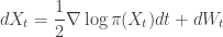
has 

There are various more-or-less formal ways to see that
Similar arguments show that for any fixed positive definite matrix 

also has 
The unadjusted Langevin algorithm
Simulating exact sample paths from SDEs such as the overdamped Langevin diffusion model is typically difficult (though not necessarily impossible), so we instead want something simple and tractable as the basis of our MCMC algorithms. Here we will just simulate from the Euler–Maruyama approximation of the process by choosing a small but finite time step 

as the basis of our MCMC method. For sufficiently small
Implementation
R
We can create a kernel for the unadjusted Langevin algorithm in R with the following function.
ulKernel = function(glpi, dt = 1e-4, pre = 1) {
    sdt = sqrt(dt)
    spre = sqrt(pre)
    advance = function(x) x + 0.5*pre*glpi(x)*dt
    function(x, ll) rnorm(p, advance(x), spre*sdt)
}
Here, we can pass in pre, which is expected to be a vector representing the diagonal of the pre-conditioning matrix,
Python
def ulKernel(glpi, dt = 1e-4, pre = 1):
    p = len(init)
    sdt = np.sqrt(dt)
    spre = np.sqrt(pre)
    advance = lambda x: x + 0.5*pre*glpi(x)*dt
    def kernel(x):
        return advance(x) + np.random.randn(p)*spre*sdt
    return kernel
See the full runnable script for further details.
JAX
def ulKernel(lpi, dt = 1e-4, pre = 1):
    p = len(init)
    glpi = jit(grad(lpi))
    sdt = jnp.sqrt(dt)
    spre = jnp.sqrt(pre)
    advance = jit(lambda x: x + 0.5*pre*glpi(x)*dt)
    @jit
    def kernel(key, x):
        return advance(x) + jax.random.normal(key, [p])*spre*sdt
    return kernel
Note how for JAX we can just pass in the log posterior, and the gradient function can be obtained by automatic differentiation. See the full runnable script for further details.
Scala
def ulKernel(glp: DVD => DVD, pre: DVD, dt: Double): DVD => DVD =
  val sdt = math.sqrt(dt)
  val spre = sqrt(pre)
  def advance(beta: DVD): DVD =
    beta + (0.5*dt)*(pre*:*glp(beta))
  beta => advance(beta) + sdt*spre.map(Gaussian(0,_).sample())
See the full runnable script for further details.
Haskell
ulKernel :: (StatefulGen g m) =>
  (Vector Double -> Vector Double) -> Vector Double -> Double -> g ->
  Vector Double -> m (Vector Double)
ulKernel glpi pre dt g beta = do
  let sdt = sqrt dt
  let spre = cmap sqrt pre
  let p = size pre
  let advance beta = beta + (scalar (0.5*dt))*pre*(glpi beta)
  zl <- (replicateM p . genContVar (normalDistr 0.0 1.0)) g
  let z = fromList zl
  return $latex  advance(beta) + (scalar sdt)*spre*z
See the full runnable script for further details.
Dex
In Dex we can write a function that accepts a gradient function
def ulKernel {n} (glpi: (Fin n)=>Float -> (Fin n)=>Float)
    (pre: (Fin n)=>Float) (dt: Float)
    (b: (Fin n)=>Float) (k: Key) : (Fin n)=>Float =
  sdt = sqrt dt
  spre = sqrt pre
  b + (((0.5)*dt) .* (pre*(glpi b))) +
    (sdt .* (spre*(randn_vec k)))
or we can write a function that accepts a log posterior, and uses auto-diff to construct the gradient
def ulKernel {n} (lpi: (Fin n)=>Float -> Float)
    (pre: (Fin n)=>Float) (dt: Float)
    (b: (Fin n)=>Float) (k: Key) : (Fin n)=>Float =
  glpi = grad lpi
  sdt = sqrt dt
  spre = sqrt pre
  b + ((0.5)*dt) .* (pre*(glpi b)) +
    sdt .* (spre*(randn_vec k))
and since Dex is statically typed, we can’t easily mix these functions up.
See the full runnable scripts, without and with auto-diff.
Next steps
In this post we have seen how to construct an MCMC algorithm that makes use of gradient information. But this algorithm is approximate. In the next post we’ll see how to correct for the approximation by using the Langevin updates as proposals within a Metropolis-Hastings algorithm.

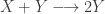

 representing the prey species and
  the predator. I showed how to simulate realisations from this process using the Scala library in the


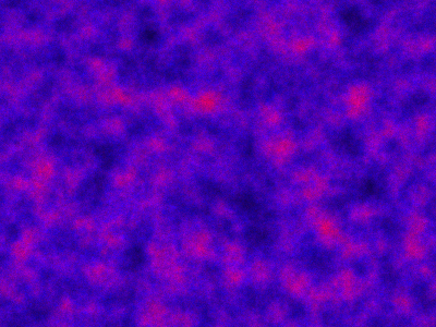


 , red
, red  and blue
  . In this simulation,