A probability monad for the bootstrap particle filter

Introduction

In the previous post I showed how to write your own general-purpose monadic probabilistic programming language from scratch in 50 lines of (Scala) code. That post is a pre-requisite for this one, so if you haven’t read it, go back and have a quick skim through it before proceeding. In that post I tried to keep everything as simple as possible, but at the expense of both elegance and efficiency. In this post I’ll address one problem with the implementation from that post – the memory (and computational) overhead associated with forming the Cartesian product of particle sets during monadic binding (flatMap). So if particle sets are typically of size , then the Cartesian product is of size , and multinomial resampling is applied to this set of size in order to sample back down to a set of size . But this isn’t actually necessary. We can directly construct a set of size , certainly saving memory, but also potentially saving computation time if the conditional distribution (on the right of the monadic bind) can be efficiently sampled. If we do this we will have a probability monad encapsulating the logic of a bootstrap particle filter, such as is often used for computing the filtering distribution of a state-space model in time series analysis. This simple change won’t solve the computational issues associated with deep monadic binding, but does solve the memory problem, and can lead to computationally efficient algorithms so long as care is taken in the formulation of probabilistic programs to ensure that deep monadic binding doesn’t occur. We’ll discuss that issue in the context of state-space models later, once we have our new SMC-based probability monad.

Materials for this post can be found in my blog repo, and a draft of this post itself can be found in the form of an executable tut document.

An SMC-based monad

The idea behind the approach to binding used in this monad is to mimic the “predict” step of a bootstrap particle filter. Here, for each particle in the source distribution, exactly one particle is drawn from the required conditional distribution and paired with the source particle, preserving the source particle’s original weight. So, in order to operationalise this, we will need a draw method adding into our probability monad. It will also simplify things to add a flatMap method to our Particle type constructor.

To follow along, you can type sbt console from the min-ppl2 directory of my blog repo, then paste blocks of code one at a time.

  import breeze.stats.{distributions => bdist}
  import breeze.linalg.DenseVector
  import cats._
  import cats.implicits._

  implicit val numParticles = 2000

  case class Particle[T](v: T, lw: Double) { // value and log-weight
    def map[S](f: T => S): Particle[S] = Particle(f(v), lw)
    def flatMap[S](f: T => Particle[S]): Particle[S] = {
      val ps = f(v)
      Particle(ps.v, lw + ps.lw)
    }
  }

I’ve added a dependence on cats here, so that we can use some derived methods, later. To take advantage of this, we must provide evidence that our custom types conform to standard type class interfaces. For example, we can provide evidence that Particle[_] is a monad as follows.

  implicit val particleMonad = new Monad[Particle] {
    def pure[T](t: T): Particle[T] = Particle(t, 0.0)
    def flatMap[T,S](pt: Particle[T])(f: T => Particle[S]): Particle[S] = pt.flatMap(f)
    def tailRecM[T,S](t: T)(f: T => Particle[Either[T,S]]): Particle[S] = ???
  }

The technical details are not important for this post, but we’ll see later what this can give us.

We can now define our Prob[_] monad in the following way.

  trait Prob[T] {
    val particles: Vector[Particle[T]]
    def draw: Particle[T]
    def mapP[S](f: T => Particle[S]): Prob[S] = Empirical(particles map (_ flatMap f))
    def map[S](f: T => S): Prob[S] = mapP(v => Particle(f(v), 0.0))
    def flatMap[S](f: T => Prob[S]): Prob[S] = mapP(f(_).draw)
    def resample(implicit N: Int): Prob[T] = {
      val lw = particles map (_.lw)
      val mx = lw reduce (math.max(_,_))
      val rw = lw map (lwi => math.exp(lwi - mx))
      val law = mx + math.log(rw.sum/(rw.length))
      val ind = bdist.Multinomial(DenseVector(rw.toArray)).sample(N)
      val newParticles = ind map (i => particles(i))
      Empirical(newParticles.toVector map (pi => Particle(pi.v, law)))
    }
    def cond(ll: T => Double): Prob[T] = mapP(v => Particle(v, ll(v)))
    def empirical: Vector[T] = resample.particles.map(_.v)
  }

  case class Empirical[T](particles: Vector[Particle[T]]) extends Prob[T] {
    def draw: Particle[T] = {
      val lw = particles map (_.lw)
      val mx = lw reduce (math.max(_,_))
      val rw = lw map (lwi => math.exp(lwi - mx))
      val law = mx + math.log(rw.sum/(rw.length))
      val idx = bdist.Multinomial(DenseVector(rw.toArray)).draw
      Particle(particles(idx).v, law)
    }
  }

As before, if you are pasting code blocks into the REPL, you will need to use :paste mode to paste these two definitions together.

The essential structure is similar to that from the previous post, but with a few notable differences. Most fundamentally, we now require any concrete implementation to provide a draw method returning a single particle from the distribution. Like before, we are not worrying about purity of functional code here, and using a standard random number generator with a globally mutating state. We can define a mapP method (for “map particle”) using the new flatMap method on Particle, and then use that to define map and flatMap for Prob[_]. Crucially, draw is used to define flatMap without requiring a Cartesian product of distributions to be formed.

We add a draw method to our Empirical[_] implementation. This method is computationally intensive, so it will still be computationally problematic to chain several flatMaps together, but this will no longer be in memory utilisation. Note that again we carefully set the weight of the drawn particle so that its raw weight is the average of the raw weight of the empirical distribution. This is needed to propagate conditioning information correctly back through flatMaps. There is obviously some code duplication between the draw method on Empirical and the resample method on Prob, but I’m not sure it’s worth factoring out.

It is worth noting that neither flatMap nor cond triggers resampling, so the user of the library is now responsible for resampling when appropriate.

We can provide evidence that Prob[_] forms a monad just like we did Particle[_].

  implicit val probMonad = new Monad[Prob] {
    def pure[T](t: T): Prob[T] = Empirical(Vector(Particle(t, 0.0)))
    def flatMap[T,S](pt: Prob[T])(f: T => Prob[S]): Prob[S] = pt.flatMap(f)
    def tailRecM[T,S](t: T)(f: T => Prob[Either[T,S]]): Prob[S] = ???
  }

Again, we’ll want to be able to create a distribution from an unweighted collection of values.

  def unweighted[T](ts: Vector[T], lw: Double = 0.0): Prob[T] =
    Empirical(ts map (Particle(_, lw)))

We will again define an implementation for distributions with tractable likelihoods, which are therefore easy to condition on. They will typically also be easy to draw from efficiently, and we will use this fact, too.

  trait Dist[T] extends Prob[T] {
    def ll(obs: T): Double
    def ll(obs: Seq[T]): Double = obs map (ll) reduce (_+_)
    def fit(obs: Seq[T]): Prob[T] = mapP(v => Particle(v, ll(obs)))
    def fitQ(obs: Seq[T]): Prob[T] = Empirical(Vector(Particle(obs.head, ll(obs))))
    def fit(obs: T): Prob[T] = fit(List(obs))
    def fitQ(obs: T): Prob[T] = fitQ(List(obs))
  }

We can give implementations of this for a few standard distributions.

  case class Normal(mu: Double, v: Double)(implicit N: Int) extends Dist[Double] {
    lazy val particles = unweighted(bdist.Gaussian(mu, math.sqrt(v)).
      sample(N).toVector).particles
    def draw = Particle(bdist.Gaussian(mu, math.sqrt(v)).draw, 0.0)
    def ll(obs: Double) = bdist.Gaussian(mu, math.sqrt(v)).logPdf(obs)
  }

  case class Gamma(a: Double, b: Double)(implicit N: Int) extends Dist[Double] {
    lazy val particles = unweighted(bdist.Gamma(a, 1.0/b).
      sample(N).toVector).particles
    def draw = Particle(bdist.Gamma(a, 1.0/b).draw, 0.0)
    def ll(obs: Double) = bdist.Gamma(a, 1.0/b).logPdf(obs)
  }

  case class Poisson(mu: Double)(implicit N: Int) extends Dist[Int] {
    lazy val particles = unweighted(bdist.Poisson(mu).
      sample(N).toVector).particles
    def draw = Particle(bdist.Poisson(mu).draw, 0.0)
    def ll(obs: Int) = bdist.Poisson(mu).logProbabilityOf(obs)
  }

Note that we now have to provide an (efficient) draw method for each implementation, returning a single draw from the distribution as a Particle with a (raw) weight of 1 (log weight of 0).

We are done. It’s a few more lines of code than that from the previous post, but this is now much closer to something that could be used in practice to solve actual inference problems using a reasonable number of particles. But to do so we will need to be careful do avoid deep monadic binding. This is easiest to explain with a concrete example.

Using the SMC-based probability monad in practice

Monadic binding and applicative structure

As explained in the previous post, using Scala’s for-expressions for monadic binding gives a natural and elegant PPL for our probability monad “for free”. This is fine, and in general there is no reason why using it should lead to inefficient code. However, for this particular probability monad implementation, it turns out that deep monadic binding comes with a huge performance penalty. For a concrete example, consider the following specification, perhaps of a prior distribution over some independent parameters.

    val prior = for {
      x <- Normal(0,1)
      y <- Gamma(1,1)
      z <- Poisson(10)
    } yield (x,y,z)

Don’t paste that into the REPL – it will take an age to complete!

Again, I must emphasise that there is nothing wrong with this specification, and there is no reason in principle why such a specification can’t be computationally efficient – it’s just a problem for our particular probability monad. We can begin to understand the problem by thinking about how this will be de-sugared by the compiler. Roughly speaking, the above will de-sugar to the following nested flatMaps.

    val prior2 =
      Normal(0,1) flatMap {x =>
        Gamma(1,1) flatMap {y =>
          Poisson(10) map {z =>
            (x,y,z)}}}

Again, beware of pasting this into the REPL.

So, although written from top to bottom, the nesting is such that the flatMaps collapse from the bottom-up. The second flatMap (the first to collapse) isn’t such a problem here, as the Poisson has a draw method. But the result is an empirical distribution, which has an draw method. So the first flatMap (the second to collapse) is an operation. By extension, it’s easy to see that the computational cost of nested flatMaps will be exponential in the number of monadic binds. So, looking back at the for expression, the problem is that there are three <-. The last one isn’t a problem since it corresponds to a map, and the second last one isn’t a problem, since the final distribution is tractable with an draw method. The problem is the first <-, corresponding to a flatMap of one empirical distribution with respect to another. For our particular probability monad, it’s best to avoid these if possible.

The interesting thing to note here is that because the distributions are independent, there is no need for them to be sequenced. They could be defined in any order. In this case it makes sense to use the applicative structure implied by the monad.

Now, since we have told cats that Prob[_] is a monad, it can provide appropriate applicative methods for us automatically. In Cats, every monad is assumed to be also an applicative functor (which is true in Cartesian closed categories, and Cats implicitly assumes that all functors and monads are defined over CCCs). So we can give an alternative specification of the above prior using applicative composition.

 val prior3 = Applicative[Prob].tuple3(Normal(0,1), Gamma(1,1), Poisson(10))
// prior3: Wrapped.Prob[(Double, Double, Int)] = Empirical(Vector(Particle((-0.057088546468105204,0.03027578552505779,9),0.0), Particle((-0.43686658266043743,0.632210127012762,14),0.0), Particle((-0.8805715148936012,3.4799656228544706,4),0.0), Particle((-0.4371726407147289,0.0010707859994652403,12),0.0), Particle((2.0283297088320755,1.040984491158822,10),0.0), Particle((1.2971862986495886,0.189166705596747,14),0.0), Particle((-1.3111333817551083,0.01962422606642761,9),0.0), Particle((1.6573851896142737,2.4021836368401415,9),0.0), Particle((-0.909927220984726,0.019595551644771683,11),0.0), Particle((0.33888133893822464,0.2659823344145805,10),0.0), Particle((-0.3300797295729375,3.2714740256437667,10),0.0), Particle((-1.8520554352884224,0.6175322756460341,10),0.0), Particle((0.541156780497547...

This one is mathematically equivalent, but safe to paste into your REPL, as it does not involve deep monadic binding, and can be used whenever we want to compose together independent components of a probabilistic program. Note that “tupling” is not the only possibility – Cats provides a range of functions for manipulating applicative values.

This is one way to avoid deep monadic binding, but another strategy is to just break up a large for expression into separate smaller for expressions. We can examine this strategy in the context of state-space modelling.

Particle filtering for a non-linear state-space model

We can now re-visit the DGLM example from the previous post. We began by declaring some observations and a prior.

    val data = List(2,1,0,2,3,4,5,4,3,2,1)
// data: List[Int] = List(2, 1, 0, 2, 3, 4, 5, 4, 3, 2, 1)

    val prior = for {
      w <- Gamma(1, 1)
      state0 <- Normal(0.0, 2.0)
    } yield (w, List(state0))
// prior: Wrapped.Prob[(Double, List[Double])] = Empirical(Vector(Particle((4.220683377724395,List(0.37256749723762683)),0.0), Particle((0.4436668049925418,List(-1.0053578391265572)),0.0), Particle((0.9868899648436931,List(-0.6985099310193449)),0.0), Particle((0.13474375773634908,List(0.9099291736792412)),0.0), Particle((1.9654021747685184,List(-0.042127103727998175)),0.0), Particle((0.21761202474220223,List(1.1074616830012525)),0.0), Particle((0.31037163527711015,List(0.9261849914020324)),0.0), Particle((1.672438830781466,List(0.01678529855289384)),0.0), Particle((0.2257151759143097,List(2.5511304854128354)),0.0), Particle((0.3046489890769499,List(3.2918304533361398)),0.0), Particle((1.5115941814057159,List(-1.633612165168878)),0.0), Particle((1.4185906813831506,List(-0.8460922678989864))...

Looking carefully at the for-expression, there are just two <-, and the distribution on the RHS of the flatMap is tractable, so this is just . So far so good.

Next, let’s look at the function to add a time point, which previously looked something like the following.

    def addTimePointSIS(current: Prob[(Double, List[Double])],
      obs: Int): Prob[(Double, List[Double])] = {
      println(s"Conditioning on observation: $obs")
      for {
        tup <- current
        (w, states) = tup
        os = states.head
        ns <- Normal(os, w)
        _ <- Poisson(math.exp(ns)).fitQ(obs)
      } yield (w, ns :: states)
    }
// addTimePointSIS: (current: Wrapped.Prob[(Double, List[Double])], obs: Int)Wrapped.Prob[(Double, List[Double])]

Recall that our new probability monad does not automatically trigger resampling, so applying this function in a fold will lead to a simple sampling importance sampling (SIS) particle filter. Typically, the bootstrap particle filter includes resampling after each time point, giving a special case of a sampling importance resampling (SIR) particle filter, which we could instead write as follows.

    def addTimePointSimple(current: Prob[(Double, List[Double])],
      obs: Int): Prob[(Double, List[Double])] = {
      println(s"Conditioning on observation: $obs")
      val updated = for {
        tup <- current
        (w, states) = tup
        os = states.head
        ns <- Normal(os, w)
        _ <- Poisson(math.exp(ns)).fitQ(obs)
      } yield (w, ns :: states)
      updated.resample
    }
// addTimePointSimple: (current: Wrapped.Prob[(Double, List[Double])], obs: Int)Wrapped.Prob[(Double, List[Double])]

This works fine, but we can see that there are three <- in this for expression. This leads to a flatMap with an empirical distribution on the RHS, and hence is . But this is simple enough to fix, by separating the updating process into separate “predict” and “update” steps, which is how people typically formulate particle filters for state-space models, anyway. Here we could write that as

    def addTimePoint(current: Prob[(Double, List[Double])],
      obs: Int): Prob[(Double, List[Double])] = {
      println(s"Conditioning on observation: $obs")
      val predict = for {
        tup <- current
        (w, states) = tup
        os = states.head
        ns <- Normal(os, w)
      }
      yield (w, ns :: states)
      val updated = for {
        tup <- predict
        (w, states) = tup
        st = states.head
        _ <- Poisson(math.exp(st)).fitQ(obs)
      } yield (w, states)
      updated.resample
    }
// addTimePoint: (current: Wrapped.Prob[(Double, List[Double])], obs: Int)Wrapped.Prob[(Double, List[Double])]

By breaking the for expression into two: the first for the “predict” step and the second for the “update” (conditioning on the observation), we get two operations, which for large is clearly much faster. We can then run the filter by folding over the observations.

  import breeze.stats.{meanAndVariance => meanVar}
// import breeze.stats.{meanAndVariance=>meanVar}

  val mod = data.foldLeft(prior)(addTimePoint(_,_)).empirical
// Conditioning on observation: 2
// Conditioning on observation: 1
// Conditioning on observation: 0
// Conditioning on observation: 2
// Conditioning on observation: 3
// Conditioning on observation: 4
// Conditioning on observation: 5
// Conditioning on observation: 4
// Conditioning on observation: 3
// Conditioning on observation: 2
// Conditioning on observation: 1
// mod: Vector[(Double, List[Double])] = Vector((0.24822528144246606,List(0.06290285371838457, 0.01633338109272575, 0.8997103339551227, 1.5058726341571411, 1.0579925693609091, 1.1616536515200064, 0.48325623593870665, 0.8457351097543767, -0.1988290999293708, -0.4787511341321954, -0.23212497417019512, -0.15327432440577277)), (1.111430233331792,List(0.6709342824443849, 0.009092797044165657, -0.13203367846117453, 0.4599952735399485, 1.3779288637042504, 0.6176597963402879, 0.6680455419800753, 0.48289163013446945, -0.5994001698510807, 0.4860969602653898, 0.10291798193078927, 1.2878325765987266)), (0.6118925941009055,List(0.6421161986636132, 0.679470360928868, 1.0552459559203342, 1.200835166087372, 1.3690372269589233, 1.8036766847282912, 0.6229883551656629, 0.14872642198313774, -0.122700856878725...

  meanVar(mod map (_._1)) // w
// res0: breeze.stats.meanAndVariance.MeanAndVariance = MeanAndVariance(0.2839184023932576,0.07391602428256917,2000)

  meanVar(mod map (_._2.reverse.head)) // initial state
// res1: breeze.stats.meanAndVariance.MeanAndVariance = MeanAndVariance(0.26057368528422714,0.4802810202354611,2000)

  meanVar(mod map (_._2.head)) // final state
// res2: breeze.stats.meanAndVariance.MeanAndVariance = MeanAndVariance(0.5448036669181697,0.28293080584600894,2000)

Summary and conclusions

Here we have just done some minor tidying up of the rather naive probability monad from the previous post to produce an SMC-based probability monad with improved performance characteristics. Again, we get an embedded probabilistic programming language “for free”. Although the language itself is very flexible, allowing us to construct more-or-less arbitrary probabilistic programs for Bayesian inference problems, we saw that a bug/feature of this particular inference algorithm is that care must be taken to avoid deep monadic binding if reasonable performance is to be obtained. In most cases this is simple to achieve by using applicative composition or by breaking up large for expressions.

There are still many issues and inefficiencies associated with this PPL. In particular, if the main intended application is to state-space models, it would make more sense to tailor the algorithms and implementations to exactly that case. OTOH, if the main concern is a generic PPL, then it would make sense to make the PPL independent of the particular inference algorithm. These are both potential topics for future posts.

Software

• min-ppl2 – code associated with this blog post
• Rainier – a more efficient PPL with similar syntax
• monad-bayes – a Haskell library exploring related ideas

Stochastic reaction-diffusion modelling

Introduction

There is a fairly large literature on reaction-diffusion modelling using partial differential equations (PDEs). There is also a fairly large literature on stochastic modelling of coupled chemical reactions, which account for the discreteness of reacting species at low concentrations. There is some literature on combining the two, to form stochastic reaction-diffusion systems, but much less.

In this post we will look at one approach to the stochastic reaction-diffusion problem, based on an underlying stochastic process often described by the reaction diffusion master equation (RDME). We will start by generating exact realisations from this process using the spatial Gillespie algorithm, before switching to a continuous stochastic approximation often known as the spatial chemical Langevin equation (spatial CLE). For fine discretisations, this spatial CLE is just an explicit numerical scheme for an associated reaction-diffusion stochastic partial differential equation (SPDE), and we can easily contrast such SPDE dynamics with their deterministic PDE approximation. We will investigate using simulation, based on my Scala library, scala-smfsb, which accompanies the third edition of my textbook, Stochastic modelling for systems biology, as discussed in previous posts.

All of the code used to generate the plots and movies in this post is available in my blog repo, and is very simple to build and run.

The Lotka-Volterra reaction network

Exact simulation from the RDME

My favourite toy coupled chemical reaction network is the Lotka-Volterra predator-prey system, presented as the three reactions

with representing the prey species and the predator. I showed how to simulate realisations from this process using the Scala library in the previous post. Here we will consider simulation of this model in 2d, and simulate exact realisation from the appropriate RDME using the spatial Gillespie algorithm. Full runnable code for this simulation is here, but the key lines are:

val r = 100; val c = 120
val model = SpnModels.lv[IntState]()
val step = Spatial.gillespie2d(model, DenseVector(0.6, 0.6), maxH=1e12)
val x00 = DenseVector(0, 0)
val x0 = DenseVector(50, 100)
val xx00 = PMatrix(r, c, Vector.fill(r*c)(x00))
val xx0 = xx00.updated(c/2, r/2, x0)
val s = Stream.iterate(xx0)(step(_,0.0,0.1))

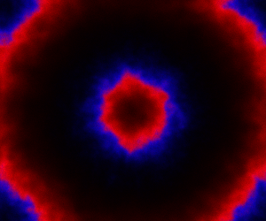
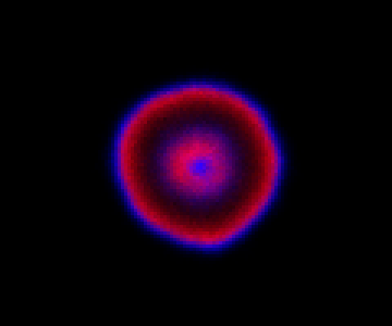
which sets up an infinite lazy Stream of states on a 100×120 grid over time steps of 0.1 units with diffusion rates of 0.6 for both species. We can then map this to a stream of images and visualise it using my scala-view library (described in this post). Running gives the following output:

The above image is the final frame of a movie which can be viewed by clicking on the image. In the simulation, blue represents the prey species, , and red represents the predator, . The simulation is initialised with a few prey and predators in the central pixel. At each time step of the simulation, either a reaction or a diffusion event may occur. If diffusion occurs, an individual moves from its current location to one of the four adjacent pixels. This algorithm is extremely computationally intensive, however well it is implemented. The implementation used here (using the function Spatial.gillespie2d in the scala-smfsb library) is quite inefficient. A more efficient implementation would use the next subvolume method or similar algorithm. But since every reaction event is simulated sequentially, this algorithm is always going to be intolerably slow for most interesting problems.

The spatial CLE

The spatial CLE effectively approximates the true RDME dynamics with a set of coupled stochastic differential equations (SDEs) on the spatial grid. This can be interpreted as an explicit scheme for numerically integrating an SPDE. But this numerical scheme is much more efficient, allowing sensible time-stepping of the process, and vectorises and parallelises nicely. The details are in my book, but the Scala implementation is here. Diffusion is implemented efficiently and in parallel using the comonadic approach that I’ve described previously. We can quickly and easily generate large simulations using the spatial CLE. Here is a movie generated on a 250×300 grid.

Again, clicking on the frame should give the movie. We see that although the quantitative details are slightly different to the exact algorithm, the essential qualitative behaviour of the system is captured well by the spatial CLE. Full code for this simulation is here.

Reaction-diffusion PDE

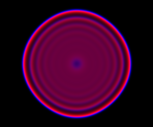
If we remove all of the noise terms from the spatial CLE, we get a set of coupled ODEs, which again, may be interpreted as a numerical scheme for integrating a reaction-diffusion PDE model. Below are the dynamics on the same 250×300 grid.

It seems a bit harsh to describe a reaction-diffusion PDE as “boring”, but it certainly isn’t as interesting as the stochastic dynamics. Also, it has qualitatively quite different behaviour to the stochastic models, with wavefronts being less pronounced and less well separated. The code for this one is here.

Other initialisations

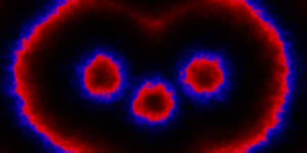
Instead of just seeding the simulation with some individuals in the central pixel, we can initialise 3 pixels. We can look first at a spatial CLE simulation.

Code here.

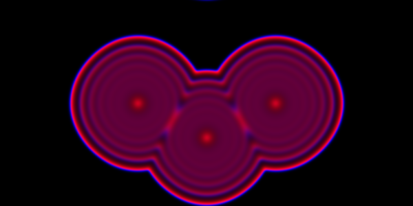
We can look at the same problem, but now using a PDE.

Code here.

Alternatively, we can initialise every pixel independently with random numbers of predator and prey. A movie for this is given below, following a short warm-up.

Code here.

Again, we can look at the corresponding deterministic integration.

Code here.

The SIR model

Let’s now turn attention to a spatial epidemic process model, the spatial susceptible-infectious-recovered model. Again, we’ll start from the discrete reaction formulation.

I’ll add this model to the next release of scala-smfsb, but in the meantime we can easily define it ourselves with:

def sir[S: State](p: DenseVector[Double] = DenseVector(0.1, 0.5)): Spn[S] =
  UnmarkedSpn[S](
    List("S", "I", "R"),
    DenseMatrix((1, 1, 0), (0, 1, 0)),
    DenseMatrix((0, 2, 0), (0, 0, 1)),
    (x, t) => {
      val xd = x.toDvd
      DenseVector(
        xd(0) * xd(1) * p(0), xd(1) * p(1)
      )}
  )

We can seed a simulation with a few infectious individuals in the centre of a roughly homogeneous population of susceptibles.

Spatial CLE

This time we’ll skip the exact simulation, since it’s very slow, and go straight to the spatial CLE. A simulation on a 250×300 grid is given below.

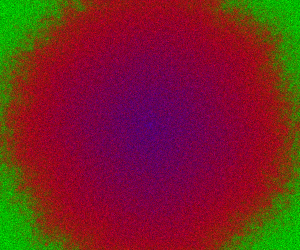
Here, green represents , red and blue . In this simulation, diffuses more slowly than , and doesn’t diffuse at all.
Code here.

PDE model

If we ditch the noise to get a reaction-diffusion PDE model, the dynamics are as follows.

Again, we see that the deterministic model is quite different to the stochastic version, and kind-of boring. Code here.

Further information

All of the code used to generate the plots and movies in this post is available in an easily runnable form in my blog repo. It is very easy to adapt the examples to vary parameters and initial conditions, and to study other reaction systems. Further details relating to stochastic reaction-diffusion modelling based on the RDME can be found in Chapter 9 of my textbook, Stochastic modelling for systems biology, third edition.

The smfsb R package

Introduction

In the previous post I gave a brief introduction to the third edition of my textbook, Stochastic modelling for systems biology. The algorithms described in the book are illustrated by implementations in R. These implementations are collected together in an R package on CRAN called smfsb. This post will provide a brief introduction to the package and its capabilities.

Installation

The package is on CRAN – see the CRAN package page for details. So the simplest way to install it is to enter

install.packages("smfsb")

at the R command prompt. This will install the latest version that is on CRAN. Once installed, the package can be loaded with

library(smfsb)

The package is well-documented, so further information can be obtained with the usual R mechanisms, such as

vignette(package="smfsb")
vignette("smfsb")
help(package="smfsb")
?StepGillespie
example(StepCLE1D)

The version of the package on CRAN is almost certainly what you want. However, the package is developed on R-Forge – see the R-Forge project page for details. So the very latest version of the package can always be installed with

install.packages("smfsb", repos="http://R-Forge.R-project.org")

if you have a reason for wanting it.

A brief tutorial

The vignette gives a quick introduction the the library, which I don’t need to repeat verbatim here. If you are new to the package, I recommend working through that before continuing. Here I’ll concentrate on some of the new features associated with the third edition.

Simulating stochastic kinetic models

Much of the book is concerned with the simulation of stochastic kinetic models using exact and approximate algorithms. Although the primary focus of the text is the application to modelling of intra-cellular processes, the methods are also appropriate for population modelling of ecological and epidemic processes. For example, we can start by simulating a simple susceptible-infectious-recovered (SIR) disease epidemic model.

set.seed(2)
data(spnModels)

stepSIR = StepGillespie(SIR)
plot(simTs(SIR$M, 0, 8, 0.05, stepSIR),
  main="Exact simulation of the SIR model")

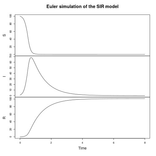
The focus of the text is stochastic simulation of discrete models, so that is the obvious place to start. But there is also support for continuous deterministic simulation.

plot(simTs(SIR$M, 0, 8, 0.05, StepEulerSPN(SIR)),
  main="Euler simulation of the SIR model")

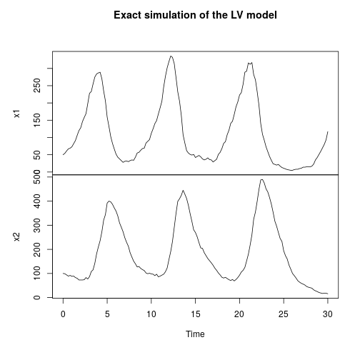
My favourite toy population dynamics model is the Lotka-Volterra (LV) model, so I tend to use this frequently as a running example throughout the book. We can simulate this (exactly) as follows.

stepLV = StepGillespie(LV)
plot(simTs(LV$M, 0, 30, 0.2, stepLV),
  main="Exact simulation of the LV model")

Stochastic reaction-diffusion modelling

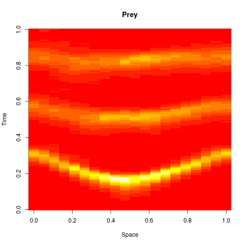
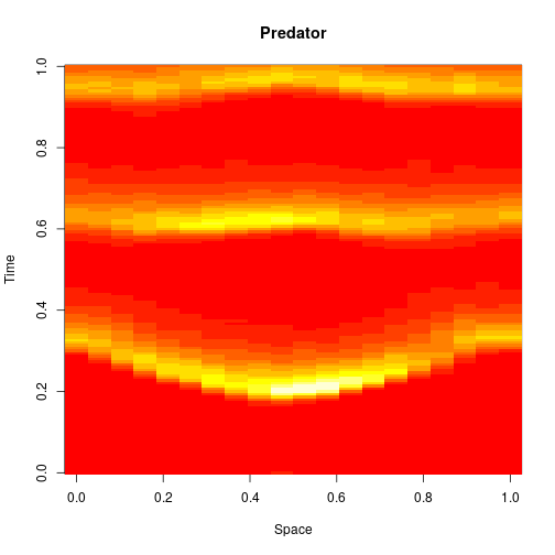
The first two editions of the book were almost exclusively concerned with well-mixed systems, where spatial effects are ignorable. One of the main new features of the third edition is the inclusion of a new chapter on spatially extended systems. The focus is on models related to the reaction diffusion master equation (RDME) formulation, rather than individual particle-based simulations. For these models, space is typically divided into a regular grid of voxels, with reactions taking place as normal within each voxel, and additional reaction events included, corresponding to the diffusion of particles to adjacent voxels. So to specify such models, we just need an initial condition, a reaction model, and diffusion coefficients (one for each reacting species). So, we can carry out exact simulation of an RDME model for a 1D spatial domain as follows.

N=20; T=30
x0=matrix(0, nrow=2, ncol=N)
rownames(x0) = c("x1", "x2")
x0[,round(N/2)] = LV$M
stepLV1D = StepGillespie1D(LV, c(0.6, 0.6))
xx = simTs1D(x0, 0, T, 0.2, stepLV1D, verb=TRUE)
image(xx[1,,], main="Prey", xlab="Space", ylab="Time")

image(xx[2,,], main="Predator", xlab="Space", ylab="Time")

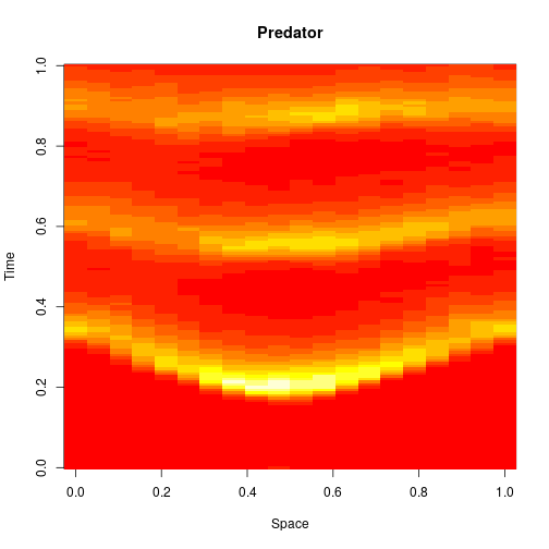
Exact simulation of discrete stochastic reaction diffusion systems is very expensive (and the reference implementation provided in the package is very inefficient), so we will often use diffusion approximations based on the CLE.

stepLV1DC = StepCLE1D(LV, c(0.6, 0.6))
xx = simTs1D(x0, 0, T, 0.2, stepLV1D)
image(xx[1,,], main="Prey", xlab="Space", ylab="Time")

image(xx[2,,], main="Predator", xlab="Space", ylab="Time")

We can think of this algorithm as an explicit numerical integration of the obvious SPDE approximation to the exact model.

The package also includes support for simulation of 2D systems. Again, we can use the Spatial CLE to speed things up.

m=70; n=50; T=10
data(spnModels)
x0=array(0, c(2,m,n))
dimnames(x0)[[1]]=c("x1", "x2")
x0[,round(m/2),round(n/2)] = LV$M
stepLV2D = StepCLE2D(LV, c(0.6,0.6), dt=0.05)
xx = simTs2D(x0, 0, T, 0.5, stepLV2D)
N = dim(xx)[4]
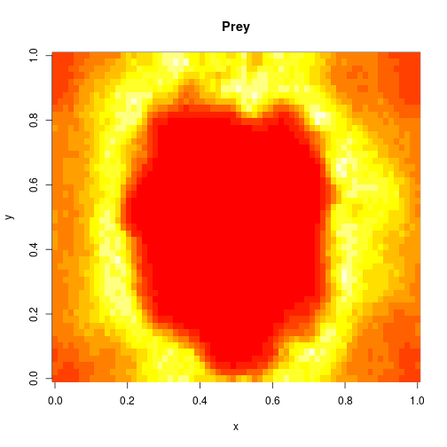
image(xx[1,,,N],main="Prey",xlab="x",ylab="y")

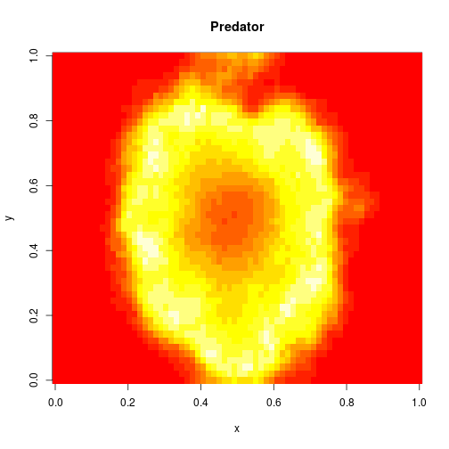
image(xx[2,,,N],main="Predator",xlab="x",ylab="y")

Bayesian parameter inference

Although much of the book is concerned with the problem of forward simulation, the final chapters are concerned with the inverse problem of estimating model parameters, such as reaction rate constants, from data. A computational Bayesian approach is adopted, with the main emphasis being placed on “likelihood free” methods, which rely on forward simulation to avoid explicit computation of sample path likelihoods. The second edition included some rudimentary code for a likelihood free particle marginal Metropolis-Hastings (PMMH) particle Markov chain Monte Carlo (pMCMC) algorithm. The third edition includes a more complete and improved implementation, in addition to approximate inference algorithms based on approximate Bayesian computation (ABC).

The key function underpinning the PMMH approach is pfMLLik, which computes an estimate of marginal model log-likelihood using a (bootstrap) particle filter. There is a new implementation of this function with the third edition. There is also a generic implementation of the Metropolis-Hastings algorithm, metropolisHastings, which can be combined with pfMLLik to create a PMMH algorithm. PMMH algorithms are very slow, but a full demo of how to use these functions for parameter inference is included in the package and can be run with

demo(PMCMC)

Simple rejection-based ABC methods are facilitated by the (very simple) function abcRun, which just samples from a prior and then carries out independent simulations in parallel before computing summary statistics. A simple illustration of the use of the function is given below.

data(LVdata)
rprior <- function() { exp(c(runif(1, -3, 3),runif(1,-8,-2),runif(1,-4,2))) }
rmodel <- function(th) { simTs(c(50,100), 0, 30, 2, stepLVc, th) }
sumStats <- identity
ssd = sumStats(LVperfect)
distance <- function(s) {
    diff = s - ssd
    sqrt(sum(diff*diff))
}
rdist <- function(th) { distance(sumStats(rmodel(th))) }
out = abcRun(10000, rprior, rdist)
q=quantile(out$dist, c(0.01, 0.05, 0.1))
print(q)

##       1%       5%      10% 
## 772.5546 845.8879 881.0573

accepted = out$param[out$dist < q[1],]
print(summary(accepted))

##        V1                V2                  V3         
##  Min.   :0.06498   Min.   :0.0004467   Min.   :0.01887  
##  1st Qu.:0.16159   1st Qu.:0.0012598   1st Qu.:0.04122  
##  Median :0.35750   Median :0.0023488   Median :0.14664  
##  Mean   :0.68565   Mean   :0.0046887   Mean   :0.36726  
##  3rd Qu.:0.86708   3rd Qu.:0.0057264   3rd Qu.:0.36870  
##  Max.   :4.76773   Max.   :0.0309364   Max.   :3.79220

print(summary(log(accepted)))

##        V1                V2               V3         
##  Min.   :-2.7337   Min.   :-7.714   Min.   :-3.9702  
##  1st Qu.:-1.8228   1st Qu.:-6.677   1st Qu.:-3.1888  
##  Median :-1.0286   Median :-6.054   Median :-1.9198  
##  Mean   :-0.8906   Mean   :-5.877   Mean   :-1.9649  
##  3rd Qu.:-0.1430   3rd Qu.:-5.163   3rd Qu.:-0.9978  
##  Max.   : 1.5619   Max.   :-3.476   Max.   : 1.3329

Naive rejection-based ABC algorithms are notoriously inefficient, so the library also includes an implementation of a more efficient, sequential version of ABC, often known as ABC-SMC, in the function abcSmc. This function requires specification of a perturbation kernel to “noise up” the particles at each algorithm sweep. Again, the implementation is parallel, using the parallel package to run the required simulations in parallel on multiple cores. A simple illustration of use is given below.

rprior <- function() { c(runif(1, -3, 3), runif(1, -8, -2), runif(1, -4, 2)) }
dprior <- function(x, ...) { dunif(x[1], -3, 3, ...) + 
    dunif(x[2], -8, -2, ...) + dunif(x[3], -4, 2, ...) }
rmodel <- function(th) { simTs(c(50,100), 0, 30, 2, stepLVc, exp(th)) }
rperturb <- function(th){th + rnorm(3, 0, 0.5)}
dperturb <- function(thNew, thOld, ...){sum(dnorm(thNew, thOld, 0.5, ...))}
sumStats <- identity
ssd = sumStats(LVperfect)
distance <- function(s) {
    diff = s - ssd
    sqrt(sum(diff*diff))
}
rdist <- function(th) { distance(sumStats(rmodel(th))) }
out = abcSmc(5000, rprior, dprior, rdist, rperturb,
    dperturb, verb=TRUE, steps=6, factor=5)

## 6 5 4 3 2 1

print(summary(out))

##        V1                V2               V3        
##  Min.   :-2.9961   Min.   :-7.988   Min.   :-3.999  
##  1st Qu.:-1.9001   1st Qu.:-6.786   1st Qu.:-3.428  
##  Median :-1.2571   Median :-6.167   Median :-2.433  
##  Mean   :-1.0789   Mean   :-6.014   Mean   :-2.196  
##  3rd Qu.:-0.2682   3rd Qu.:-5.261   3rd Qu.:-1.161  
##  Max.   : 2.1128   Max.   :-2.925   Max.   : 1.706

We can then plot some results with

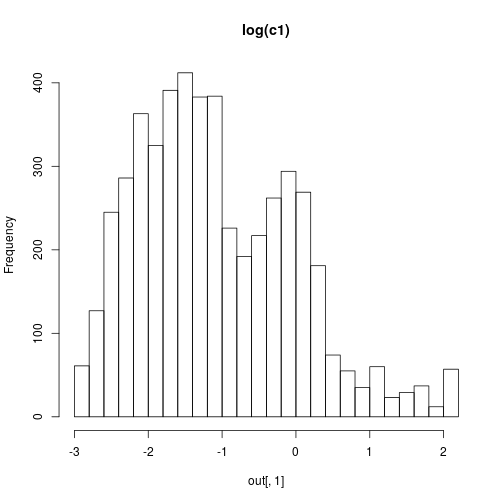
hist(out[,1],30,main="log(c1)")

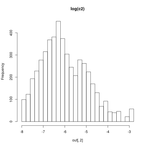
hist(out[,2],30,main="log(c2)")

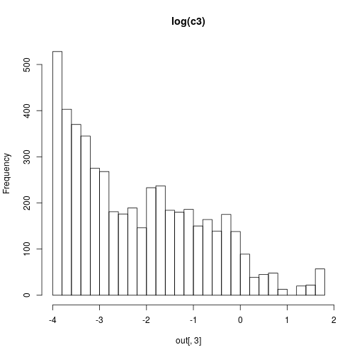
hist(out[,3],30,main="log(c3)")

Although the inference methods are illustrated in the book in the context of parameter inference for stochastic kinetic models, their implementation is generic, and can be used with any appropriate parameter inference problem.

The smfsbSBML package

smfsbSBML is another R package associated with the third edition of the book. This package is not on CRAN due to its dependency on a package not on CRAN, and hence is slightly less straightforward to install. Follow the available installation instructions to install the package. Once installed, you should be able to load the package with

library(smfsbSBML)

This package provides a function for reading in SBML files and parsing them into the simulatable stochastic Petri net (SPN) objects used by the main smfsb R package. Examples of suitable SBML models are included in the main smfsb GitHub repo. An appropriate SBML model can be read and parsed with a command like:

model = sbml2spn("mySbmlModel.xml")

The resulting value, model is an SPN object which can be passed in to simulation functions such as StepGillespie for constructing stochastic simulation algorithms.

Other software

In addition to the above R packages, I also have some Python scripts for converting between SBML and the SBML-shorthand notation I use in the book. See the SBML-shorthand page for further details.

Although R is a convenient language for teaching and learning about stochastic simulation, it isn’t ideal for serious research-level scientific computing or computational statistics. So for the third edition of the book I have also developed scala-smfsb, a library written in the Scala programming language, which re-implements all of the models and algorithms from the third edition of the book in Scala, a fast, efficient, strongly-typed, compiled, functional programming language. I’ll give an introduction to this library in a subsequent post, but in the meantime, it is already well documented, so see the scala-smfsb repo for further details, including information on installation, getting started, a tutorial, examples, API docs, etc.

Source

This blog post started out as an RMarkdown document, the source of which can be found here.