Introduction
In the previous post I gave a brief introduction to the third edition of my textbook, Stochastic modelling for systems biology. The algorithms described in the book are illustrated by implementations in R. These implementations are collected together in an R package on CRAN called smfsb. This post will provide a brief introduction to the package and its capabilities.
Installation
The package is on CRAN – see the CRAN package page for details. So the simplest way to install it is to enter
install.packages("smfsb")
at the R command prompt. This will install the latest version that is on CRAN. Once installed, the package can be loaded with
library(smfsb)
The package is well-documented, so further information can be obtained with the usual R mechanisms, such as
vignette(package="smfsb")
vignette("smfsb")
help(package="smfsb")
?StepGillespie
example(StepCLE1D)
The version of the package on CRAN is almost certainly what you want. However, the package is developed on R-Forge – see the R-Forge project page for details. So the very latest version of the package can always be installed with
install.packages("smfsb", repos="http://R-Forge.R-project.org")
if you have a reason for wanting it.
A brief tutorial
The vignette gives a quick introduction the the library, which I don’t need to repeat verbatim here. If you are new to the package, I recommend working through that before continuing. Here I’ll concentrate on some of the new features associated with the third edition.
Simulating stochastic kinetic models
Much of the book is concerned with the simulation of stochastic kinetic models using exact and approximate algorithms. Although the primary focus of the text is the application to modelling of intra-cellular processes, the methods are also appropriate for population modelling of ecological and epidemic processes. For example, we can start by simulating a simple susceptible-infectious-recovered (SIR) disease epidemic model.
set.seed(2)
data(spnModels)

stepSIR = StepGillespie(SIR)
plot(simTs(SIR$M, 0, 8, 0.05, stepSIR),
  main="Exact simulation of the SIR model")

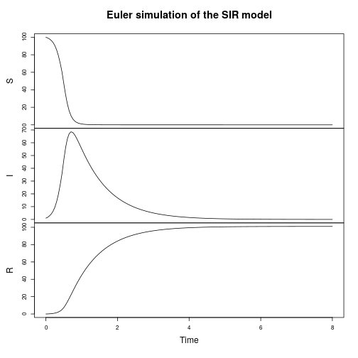
The focus of the text is stochastic simulation of discrete models, so that is the obvious place to start. But there is also support for continuous deterministic simulation.
plot(simTs(SIR$M, 0, 8, 0.05, StepEulerSPN(SIR)),
  main="Euler simulation of the SIR model")
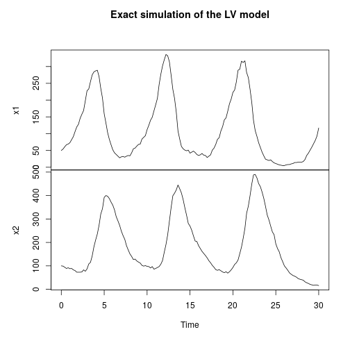
My favourite toy population dynamics model is the Lotka-Volterra (LV) model, so I tend to use this frequently as a running example throughout the book. We can simulate this (exactly) as follows.
stepLV = StepGillespie(LV)
plot(simTs(LV$M, 0, 30, 0.2, stepLV),
  main="Exact simulation of the LV model")
Stochastic reaction-diffusion modelling
The first two editions of the book were almost exclusively concerned with well-mixed systems, where spatial effects are ignorable. One of the main new features of the third edition is the inclusion of a new chapter on spatially extended systems. The focus is on models related to the reaction diffusion master equation (RDME) formulation, rather than individual particle-based simulations. For these models, space is typically divided into a regular grid of voxels, with reactions taking place as normal within each voxel, and additional reaction events included, corresponding to the diffusion of particles to adjacent voxels. So to specify such models, we just need an initial condition, a reaction model, and diffusion coefficients (one for each reacting species). So, we can carry out exact simulation of an RDME model for a 1D spatial domain as follows.
N=20; T=30
x0=matrix(0, nrow=2, ncol=N)
rownames(x0) = c("x1", "x2")
x0[,round(N/2)] = LV$M
stepLV1D = StepGillespie1D(LV, c(0.6, 0.6))
xx = simTs1D(x0, 0, T, 0.2, stepLV1D, verb=TRUE)
image(xx[1,,], main="Prey", xlab="Space", ylab="Time")
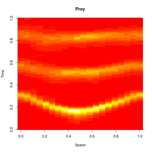
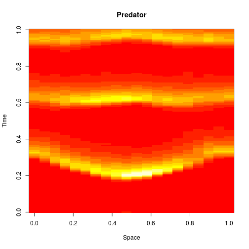
image(xx[2,,], main="Predator", xlab="Space", ylab="Time")
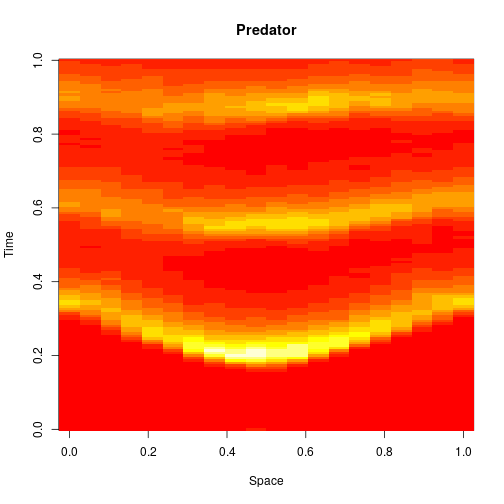
Exact simulation of discrete stochastic reaction diffusion systems is very expensive (and the reference implementation provided in the package is very inefficient), so we will often use diffusion approximations based on the CLE.
stepLV1DC = StepCLE1D(LV, c(0.6, 0.6))
xx = simTs1D(x0, 0, T, 0.2, stepLV1D)
image(xx[1,,], main="Prey", xlab="Space", ylab="Time")

image(xx[2,,], main="Predator", xlab="Space", ylab="Time")
We can think of this algorithm as an explicit numerical integration of the obvious SPDE approximation to the exact model.
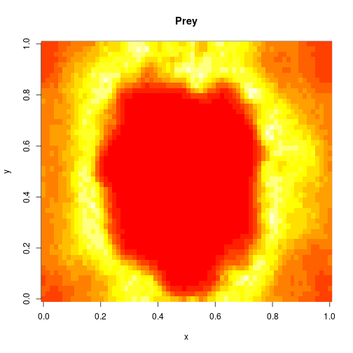
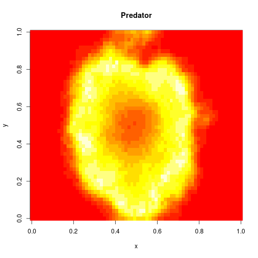
The package also includes support for simulation of 2D systems. Again, we can use the Spatial CLE to speed things up.
m=70; n=50; T=10
data(spnModels)
x0=array(0, c(2,m,n))
dimnames(x0)[[1]]=c("x1", "x2")
x0[,round(m/2),round(n/2)] = LV$M
stepLV2D = StepCLE2D(LV, c(0.6,0.6), dt=0.05)
xx = simTs2D(x0, 0, T, 0.5, stepLV2D)
N = dim(xx)[4]
image(xx[1,,,N],main="Prey",xlab="x",ylab="y")
image(xx[2,,,N],main="Predator",xlab="x",ylab="y")
Bayesian parameter inference
Although much of the book is concerned with the problem of forward simulation, the final chapters are concerned with the inverse problem of estimating model parameters, such as reaction rate constants, from data. A computational Bayesian approach is adopted, with the main emphasis being placed on “likelihood free” methods, which rely on forward simulation to avoid explicit computation of sample path likelihoods. The second edition included some rudimentary code for a likelihood free particle marginal Metropolis-Hastings (PMMH) particle Markov chain Monte Carlo (pMCMC) algorithm. The third edition includes a more complete and improved implementation, in addition to approximate inference algorithms based on approximate Bayesian computation (ABC).
The key function underpinning the PMMH approach is pfMLLik, which computes an estimate of marginal model log-likelihood using a (bootstrap) particle filter. There is a new implementation of this function with the third edition. There is also a generic implementation of the Metropolis-Hastings algorithm, metropolisHastings, which can be combined with pfMLLik to create a PMMH algorithm. PMMH algorithms are very slow, but a full demo of how to use these functions for parameter inference is included in the package and can be run with
demo(PMCMC)
Simple rejection-based ABC methods are facilitated by the (very simple) function abcRun, which just samples from a prior and then carries out independent simulations in parallel before computing summary statistics. A simple illustration of the use of the function is given below.
data(LVdata)
rprior <- function() { exp(c(runif(1, -3, 3),runif(1,-8,-2),runif(1,-4,2))) }
rmodel <- function(th) { simTs(c(50,100), 0, 30, 2, stepLVc, th) }
sumStats <- identity
ssd = sumStats(LVperfect)
distance <- function(s) {
    diff = s - ssd
    sqrt(sum(diff*diff))
}
rdist <- function(th) { distance(sumStats(rmodel(th))) }
out = abcRun(10000, rprior, rdist)
q=quantile(out$dist, c(0.01, 0.05, 0.1))
print(q)
##       1%       5%      10%
## 772.5546 845.8879 881.0573
accepted = out$param[out$dist < q[1],]
print(summary(accepted))
##        V1                V2                  V3
##  Min.   :0.06498   Min.   :0.0004467   Min.   :0.01887
##  1st Qu.:0.16159   1st Qu.:0.0012598   1st Qu.:0.04122
##  Median :0.35750   Median :0.0023488   Median :0.14664
##  Mean   :0.68565   Mean   :0.0046887   Mean   :0.36726
##  3rd Qu.:0.86708   3rd Qu.:0.0057264   3rd Qu.:0.36870
##  Max.   :4.76773   Max.   :0.0309364   Max.   :3.79220
print(summary(log(accepted)))
##        V1                V2               V3
##  Min.   :-2.7337   Min.   :-7.714   Min.   :-3.9702
##  1st Qu.:-1.8228   1st Qu.:-6.677   1st Qu.:-3.1888
##  Median :-1.0286   Median :-6.054   Median :-1.9198
##  Mean   :-0.8906   Mean   :-5.877   Mean   :-1.9649
##  3rd Qu.:-0.1430   3rd Qu.:-5.163   3rd Qu.:-0.9978
##  Max.   : 1.5619   Max.   :-3.476   Max.   : 1.3329
Naive rejection-based ABC algorithms are notoriously inefficient, so the library also includes an implementation of a more efficient, sequential version of ABC, often known as ABC-SMC, in the function abcSmc. This function requires specification of a perturbation kernel to “noise up” the particles at each algorithm sweep. Again, the implementation is parallel, using the parallel package to run the required simulations in parallel on multiple cores. A simple illustration of use is given below.
rprior <- function() { c(runif(1, -3, 3), runif(1, -8, -2), runif(1, -4, 2)) }
dprior <- function(x, ...) { dunif(x[1], -3, 3, ...) +
    dunif(x[2], -8, -2, ...) + dunif(x[3], -4, 2, ...) }
rmodel <- function(th) { simTs(c(50,100), 0, 30, 2, stepLVc, exp(th)) }
rperturb <- function(th){th + rnorm(3, 0, 0.5)}
dperturb <- function(thNew, thOld, ...){sum(dnorm(thNew, thOld, 0.5, ...))}
sumStats <- identity
ssd = sumStats(LVperfect)
distance <- function(s) {
    diff = s - ssd
    sqrt(sum(diff*diff))
}
rdist <- function(th) { distance(sumStats(rmodel(th))) }
out = abcSmc(5000, rprior, dprior, rdist, rperturb,
    dperturb, verb=TRUE, steps=6, factor=5)
## 6 5 4 3 2 1
print(summary(out))
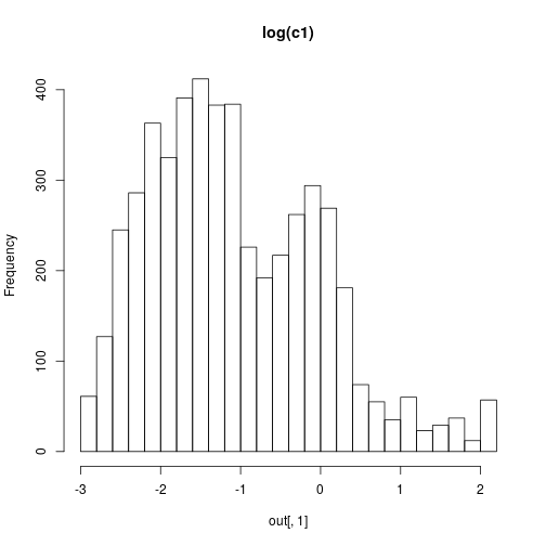
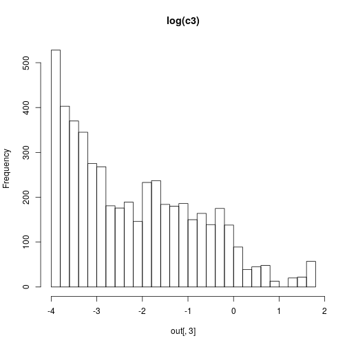
##        V1                V2               V3
##  Min.   :-2.9961   Min.   :-7.988   Min.   :-3.999
##  1st Qu.:-1.9001   1st Qu.:-6.786   1st Qu.:-3.428
##  Median :-1.2571   Median :-6.167   Median :-2.433
##  Mean   :-1.0789   Mean   :-6.014   Mean   :-2.196
##  3rd Qu.:-0.2682   3rd Qu.:-5.261   3rd Qu.:-1.161
##  Max.   : 2.1128   Max.   :-2.925   Max.   : 1.706
We can then plot some results with
hist(out[,1],30,main="log(c1)")
hist(out[,2],30,main="log(c2)")
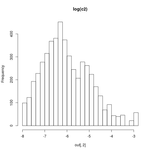
hist(out[,3],30,main="log(c3)")
Although the inference methods are illustrated in the book in the context of parameter inference for stochastic kinetic models, their implementation is generic, and can be used with any appropriate parameter inference problem.
The smfsbSBML package
smfsbSBML is another R package associated with the third edition of the book. This package is not on CRAN due to its dependency on a package not on CRAN, and hence is slightly less straightforward to install. Follow the available installation instructions to install the package. Once installed, you should be able to load the package with
library(smfsbSBML)
This package provides a function for reading in SBML files and parsing them into the simulatable stochastic Petri net (SPN) objects used by the main smfsb R package. Examples of suitable SBML models are included in the main smfsb GitHub repo. An appropriate SBML model can be read and parsed with a command like:
model = sbml2spn("mySbmlModel.xml")
The resulting value, model is an SPN object which can be passed in to simulation functions such as StepGillespie for constructing stochastic simulation algorithms.
Other software
In addition to the above R packages, I also have some Python scripts for converting between SBML and the SBML-shorthand notation I use in the book. See the SBML-shorthand page for further details.
Although R is a convenient language for teaching and learning about stochastic simulation, it isn’t ideal for serious research-level scientific computing or computational statistics. So for the third edition of the book I have also developed scala-smfsb, a library written in the Scala programming language, which re-implements all of the models and algorithms from the third edition of the book in Scala, a fast, efficient, strongly-typed, compiled, functional programming language. I’ll give an introduction to this library in a subsequent post, but in the meantime, it is already well documented, so see the scala-smfsb repo for further details, including information on installation, getting started, a tutorial, examples, API docs, etc.
Source
This blog post started out as an RMarkdown document, the source of which can be found here.

 and the predator
  as a stochastic network, viz


 ,
,  at time 0, use
