Stochastic reaction-diffusion modelling

Introduction

There is a fairly large literature on reaction-diffusion modelling using partial differential equations (PDEs). There is also a fairly large literature on stochastic modelling of coupled chemical reactions, which account for the discreteness of reacting species at low concentrations. There is some literature on combining the two, to form stochastic reaction-diffusion systems, but much less.

In this post we will look at one approach to the stochastic reaction-diffusion problem, based on an underlying stochastic process often described by the reaction diffusion master equation (RDME). We will start by generating exact realisations from this process using the spatial Gillespie algorithm, before switching to a continuous stochastic approximation often known as the spatial chemical Langevin equation (spatial CLE). For fine discretisations, this spatial CLE is just an explicit numerical scheme for an associated reaction-diffusion stochastic partial differential equation (SPDE), and we can easily contrast such SPDE dynamics with their deterministic PDE approximation. We will investigate using simulation, based on my Scala library, scala-smfsb, which accompanies the third edition of my textbook, Stochastic modelling for systems biology, as discussed in previous posts.

All of the code used to generate the plots and movies in this post is available in my blog repo, and is very simple to build and run.

The Lotka-Volterra reaction network

Exact simulation from the RDME

My favourite toy coupled chemical reaction network is the Lotka-Volterra predator-prey system, presented as the three reactions

X \longrightarrow 2X
X + Y \longrightarrow 2Y
Y \longrightarrow \emptyset

with X representing the prey species and Y the predator. I showed how to simulate realisations from this process using the Scala library in the previous post. Here we will consider simulation of this model in 2d, and simulate exact realisation from the appropriate RDME using the spatial Gillespie algorithm. Full runnable code for this simulation is here, but the key lines are:

val r = 100; val c = 120
val model = SpnModels.lv[IntState]()
val step = Spatial.gillespie2d(model, DenseVector(0.6, 0.6), maxH=1e12)
val x00 = DenseVector(0, 0)
val x0 = DenseVector(50, 100)
val xx00 = PMatrix(r, c, Vector.fill(r*c)(x00))
val xx0 = xx00.updated(c/2, r/2, x0)
val s = Stream.iterate(xx0)(step(_,0.0,0.1))

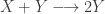
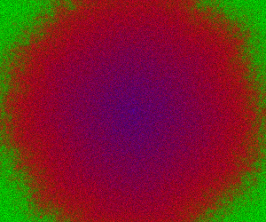
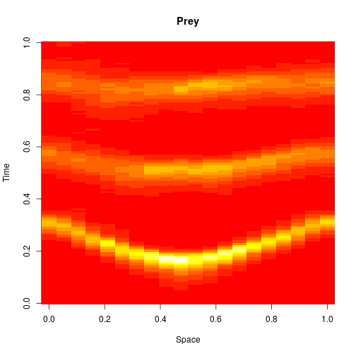
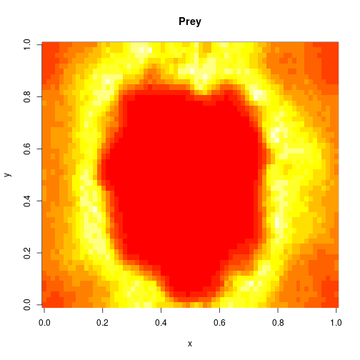
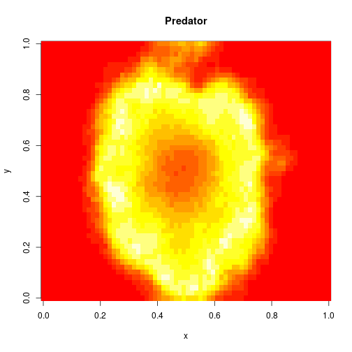
which sets up an infinite lazy Stream of states on a 100×120 grid over time steps of 0.1 units with diffusion rates of 0.6 for both species. We can then map this to a stream of images and visualise it using my scala-view library (described in this post). Running gives the following output:

Movie

The above image is the final frame of a movie which can be viewed by clicking on the image. In the simulation, blue represents the prey species, X, and red represents the predator, Y. The simulation is initialised with a few prey and predators in the central pixel. At each time step of the simulation, either a reaction or a diffusion event may occur. If diffusion occurs, an individual moves from its current location to one of the four adjacent pixels. This algorithm is extremely computationally intensive, however well it is implemented. The implementation used here (using the function Spatial.gillespie2d in the scala-smfsb library) is quite inefficient. A more efficient implementation would use the next subvolume method or similar algorithm. But since every reaction event is simulated sequentially, this algorithm is always going to be intolerably slow for most interesting problems.

The spatial CLE

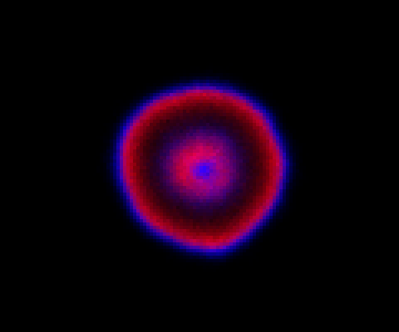
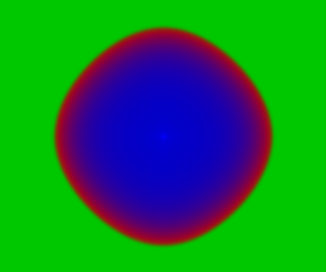
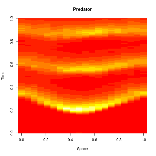
The spatial CLE effectively approximates the true RDME dynamics with a set of coupled stochastic differential equations (SDEs) on the spatial grid. This can be interpreted as an explicit scheme for numerically integrating an SPDE. But this numerical scheme is much more efficient, allowing sensible time-stepping of the process, and vectorises and parallelises nicely. The details are in my book, but the Scala implementation is here. Diffusion is implemented efficiently and in parallel using the comonadic approach that I’ve described previously. We can quickly and easily generate large simulations using the spatial CLE. Here is a movie generated on a 250×300 grid.

Movie

Again, clicking on the frame should give the movie. We see that although the quantitative details are slightly different to the exact algorithm, the essential qualitative behaviour of the system is captured well by the spatial CLE. Full code for this simulation is here.

Reaction-diffusion PDE

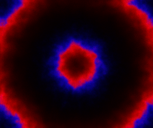
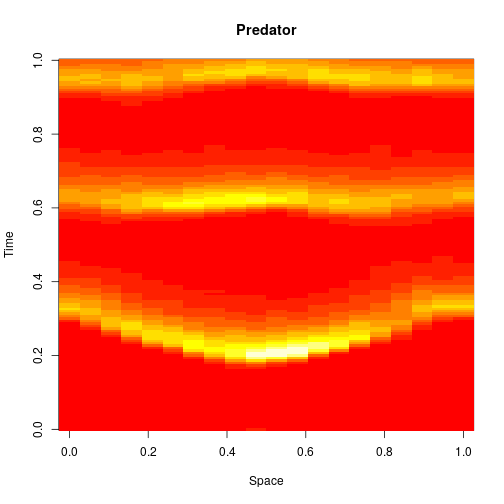
If we remove all of the noise terms from the spatial CLE, we get a set of coupled ODEs, which again, may be interpreted as a numerical scheme for integrating a reaction-diffusion PDE model. Below are the dynamics on the same 250×300 grid.

Movie

It seems a bit harsh to describe a reaction-diffusion PDE as “boring”, but it certainly isn’t as interesting as the stochastic dynamics. Also, it has qualitatively quite different behaviour to the stochastic models, with wavefronts being less pronounced and less well separated. The code for this one is here.

Other initialisations

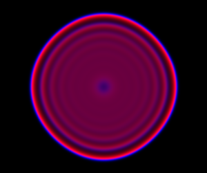
Instead of just seeding the simulation with some individuals in the central pixel, we can initialise 3 pixels. We can look first at a spatial CLE simulation.
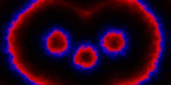
Movie

Code here.

We can look at the same problem, but now using a PDE.
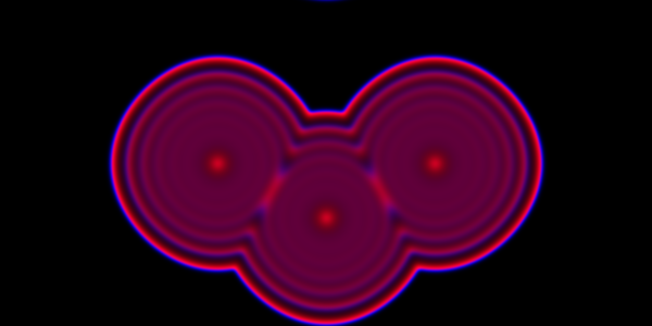
Movie

Code here.

Alternatively, we can initialise every pixel independently with random numbers of predator and prey. A movie for this is given below, following a short warm-up.
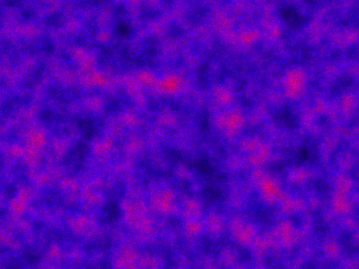
Movie

Code here.

Again, we can look at the corresponding deterministic integration.
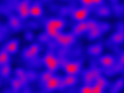
Movie

Code here.

The SIR model

Let’s now turn attention to a spatial epidemic process model, the spatial susceptible-infectious-recovered model. Again, we’ll start from the discrete reaction formulation.

S + I \longrightarrow 2I
I \longrightarrow R

I’ll add this model to the next release of scala-smfsb, but in the meantime we can easily define it ourselves with:

def sir[S: State](p: DenseVector[Double] = DenseVector(0.1, 0.5)): Spn[S] =
  UnmarkedSpn[S](
    List("S", "I", "R"),
    DenseMatrix((1, 1, 0), (0, 1, 0)),
    DenseMatrix((0, 2, 0), (0, 0, 1)),
    (x, t) => {
      val xd = x.toDvd
      DenseVector(
        xd(0) * xd(1) * p(0), xd(1) * p(1)
      )}
  )

We can seed a simulation with a few infectious individuals in the centre of a roughly homogeneous population of susceptibles.

Spatial CLE

This time we’ll skip the exact simulation, since it’s very slow, and go straight to the spatial CLE. A simulation on a 250×300 grid is given below.

Movie

Here, green represents S, red I and blue R. In this simulation, I diffuses more slowly than S, and R doesn’t diffuse at all.
Code here.

PDE model

If we ditch the noise to get a reaction-diffusion PDE model, the dynamics are as follows.

Movie

Again, we see that the deterministic model is quite different to the stochastic version, and kind-of boring. Code here.

Further information

All of the code used to generate the plots and movies in this post is available in an easily runnable form in my blog repo. It is very easy to adapt the examples to vary parameters and initial conditions, and to study other reaction systems. Further details relating to stochastic reaction-diffusion modelling based on the RDME can be found in Chapter 9 of my textbook, Stochastic modelling for systems biology, third edition.

The scala-smfsb library

In the previous post I gave a very quick introduction to the smfsb R package. As mentioned in that post, although good for teaching and learning, R isn’t a great language for serious scientific computing or computational statistics. So for the publication of the third edition of my textbook, Stochastic modelling for systems biology, I have created a library in the Scala programming language replicating the functionality provided by the R package. Here I will give a very quick introduction to the scala-smfsb library. Some familiarity with both Scala and the smfsb R package will be helpful, but is not strictly necessary. Note that the library relies on the Scala Breeze library for linear algebra and probability distributions, so some familiarity with that library can also be helpful.

Setup

To follow the along you need to have Sbt installed, and this in turn requires a recent JDK. If you are new to Scala, you may find the setup page for my Scala course to be useful, but note that on many Linux systems it can be as simple as installing the packages openjdk-8-jdk and sbt.

Once you have Sbt installed, you should be able to run it by entering sbt at your OS command line. You now need to use Sbt to create a Scala REPL with a dependency on the scala-smfsb library. There are many ways to do this, but if you are new to Scala, the simplest way is probably to start up Sbt from an empty or temporary directory (which doesn’t contain any Scala code), and then paste the following into the Sbt prompt:

set libraryDependencies += "com.github.darrenjw" %% "scala-smfsb" % "0.6"
set libraryDependencies += "org.scalanlp" %% "breeze-viz" % "0.13.2"
set scalaVersion := "2.12.6"
set scalacOptions += "-Yrepl-class-based"
console

The first time you run this it will take a little while to download and cache various library dependencies. But everything is cached, so it should be much quicker in future. When it is finished, you should have a Scala REPL ready to enter Scala code.

An introduction to scala-smfsb

It should be possible to type or copy-and-paste the commands below one-at-a-time into the Scala REPL. We need to start with a few imports.

import smfsb._
import breeze.linalg.{Vector => BVec, _}
import breeze.numerics._
import breeze.plot._

Note that I’ve renamed Breeze’s Vector type to BVec to avoid clashing with that in the Scala standard library. We are now ready to go.

Simulating models

Let’s begin by instantiating a Lotka-Volterra model, simulating a single realisation of the process, and then plotting it.

// Simulate LV with Gillespie
val model = SpnModels.lv[IntState]()
val step = Step.gillespie(model)
val ts = Sim.ts(DenseVector(50, 100), 0.0, 20.0, 0.05, step)
Sim.plotTs(ts, "Gillespie simulation of LV model with default parameters")

The library comes with a few other models. There’s a Michaelis-Menten enzyme kinetics model:

// Simulate other models with Gillespie
val stepMM = Step.gillespie(SpnModels.mm[IntState]())
val tsMM = Sim.ts(DenseVector(301,120,0,0), 0.0, 100.0, 0.5, stepMM)
Sim.plotTs(tsMM, "Gillespie simulation of the MM model")

and an auto-regulatory genetic network model, for example.

val stepAR = Step.gillespie(SpnModels.ar[IntState]())
val tsAR = Sim.ts(DenseVector(10, 0, 0, 0, 0), 0.0, 500.0, 0.5, stepAR)
Sim.plotTs(tsAR, "Gillespie simulation of the AR model")

If you know the book and/or the R package, these models should all be familiar.
We are not restricted to exact stochastic simulation using the Gillespie algorithm. We can use an approximate Poisson time-stepping algorithm.

// Simulate LV with other algorithms
val stepPts = Step.pts(model)
val tsPts = Sim.ts(DenseVector(50, 100), 0.0, 20.0, 0.05, stepPts)
Sim.plotTs(tsPts, "Poisson time-step simulation of the LV model")

Alternatively, we can instantiate the example models using a continuous state rather than a discrete state, and then simulate using algorithms based on continous approximations, such as Euler-Maruyama simulation of a chemical Langevin equation (CLE) approximation.

val stepCle = Step.cle(SpnModels.lv[DoubleState]())
val tsCle = Sim.ts(DenseVector(50.0, 100.0), 0.0, 20.0, 0.05, stepCle)
Sim.plotTs(tsCle, "Euler-Maruyama/CLE simulation of the LV model")

If we want to ignore noise temporarily, there’s also a simple continuous deterministic Euler integrator built-in.

val stepE = Step.euler(SpnModels.lv[DoubleState]())
val tsE = Sim.ts(DenseVector(50.0, 100.0), 0.0, 20.0, 0.05, stepE)
Sim.plotTs(tsE, "Continuous-deterministic Euler simulation of the LV model")

Spatial stochastic reaction-diffusion simulation

We can do 1d reaction-diffusion simulation with something like:

val N = 50; val T = 40.0
val model = SpnModels.lv[IntState]()
val step = Spatial.gillespie1d(model,DenseVector(0.8, 0.8))
val x00 = DenseVector(0, 0)
val x0 = DenseVector(50, 100)
val xx00 = Vector.fill(N)(x00)
val xx0 = xx00.updated(N/2,x0)
val output = Sim.ts(xx0, 0.0, T, 0.2, step)
Spatial.plotTs1d(output)

For 2d simulation, we use PMatrix, a comonadic matrix/image type defined within the library, with parallelised map and coflatMap (cobind) operations. See my post on comonads for scientific computing for further details on the concepts underpinning this, though note that it isn’t necessary to understand comonads to use the library.

val r = 20; val c = 30
val model = SpnModels.lv[DoubleState]()
val step = Spatial.cle2d(model, DenseVector(0.6, 0.6), 0.05)
val x00 = DenseVector(0.0, 0.0)
val x0 = DenseVector(50.0, 100.0)
val xx00 = PMatrix(r, c, Vector.fill(r*c)(x00))
val xx0 = xx00.updated(c/2, r/2, x0)
val output = step(xx0, 0.0, 8.0)
val f = Figure("2d LV reaction-diffusion simulation")
val p0 = f.subplot(2, 1, 0)
p0 += image(PMatrix.toBDM(output map (_.data(0))))
val p1 = f.subplot(2, 1, 1)
p1 += image(PMatrix.toBDM(output map (_.data(1))))

Bayesian parameter inference

The library also includes functions for carrying out parameter inference for stochastic dynamical systems models, using particle MCMC, ABC and ABC-SMC. See the examples directory for further details.

Next steps

Having worked through this post, the next step is to work through the tutorial. There is some overlap of content with this blog post, but the tutorial goes into more detail regarding the basics. It also finishes with suggestions for how to proceed further.

Source

This post started out as a tut document (the Scala equivalent of an RMarkdown document). The source can be found here.

The smfsb R package

Introduction

In the previous post I gave a brief introduction to the third edition of my textbook, Stochastic modelling for systems biology. The algorithms described in the book are illustrated by implementations in R. These implementations are collected together in an R package on CRAN called smfsb. This post will provide a brief introduction to the package and its capabilities.

Installation

The package is on CRAN – see the CRAN package page for details. So the simplest way to install it is to enter

install.packages("smfsb")

at the R command prompt. This will install the latest version that is on CRAN. Once installed, the package can be loaded with

library(smfsb)

The package is well-documented, so further information can be obtained with the usual R mechanisms, such as

vignette(package="smfsb")
vignette("smfsb")
help(package="smfsb")
?StepGillespie
example(StepCLE1D)

The version of the package on CRAN is almost certainly what you want. However, the package is developed on R-Forge – see the R-Forge project page for details. So the very latest version of the package can always be installed with

install.packages("smfsb", repos="http://R-Forge.R-project.org")

if you have a reason for wanting it.

A brief tutorial

The vignette gives a quick introduction the the library, which I don’t need to repeat verbatim here. If you are new to the package, I recommend working through that before continuing. Here I’ll concentrate on some of the new features associated with the third edition.

Simulating stochastic kinetic models

Much of the book is concerned with the simulation of stochastic kinetic models using exact and approximate algorithms. Although the primary focus of the text is the application to modelling of intra-cellular processes, the methods are also appropriate for population modelling of ecological and epidemic processes. For example, we can start by simulating a simple susceptible-infectious-recovered (SIR) disease epidemic model.

set.seed(2)
data(spnModels)

stepSIR = StepGillespie(SIR)
plot(simTs(SIR$M, 0, 8, 0.05, stepSIR),
  main="Exact simulation of the SIR model")

Exact simulation of the SIR epidemic model
The focus of the text is stochastic simulation of discrete models, so that is the obvious place to start. But there is also support for continuous deterministic simulation.

plot(simTs(SIR$M, 0, 8, 0.05, StepEulerSPN(SIR)),
  main="Euler simulation of the SIR model")

Euler simulation of the SIR model
My favourite toy population dynamics model is the Lotka-Volterra (LV) model, so I tend to use this frequently as a running example throughout the book. We can simulate this (exactly) as follows.

stepLV = StepGillespie(LV)
plot(simTs(LV$M, 0, 30, 0.2, stepLV),
  main="Exact simulation of the LV model")

Exact simulation of the Lotka-Volterra model

Stochastic reaction-diffusion modelling

The first two editions of the book were almost exclusively concerned with well-mixed systems, where spatial effects are ignorable. One of the main new features of the third edition is the inclusion of a new chapter on spatially extended systems. The focus is on models related to the reaction diffusion master equation (RDME) formulation, rather than individual particle-based simulations. For these models, space is typically divided into a regular grid of voxels, with reactions taking place as normal within each voxel, and additional reaction events included, corresponding to the diffusion of particles to adjacent voxels. So to specify such models, we just need an initial condition, a reaction model, and diffusion coefficients (one for each reacting species). So, we can carry out exact simulation of an RDME model for a 1D spatial domain as follows.

N=20; T=30
x0=matrix(0, nrow=2, ncol=N)
rownames(x0) = c("x1", "x2")
x0[,round(N/2)] = LV$M
stepLV1D = StepGillespie1D(LV, c(0.6, 0.6))
xx = simTs1D(x0, 0, T, 0.2, stepLV1D, verb=TRUE)
image(xx[1,,], main="Prey", xlab="Space", ylab="Time")

Discrete 1D simulation of the LV model

image(xx[2,,], main="Predator", xlab="Space", ylab="Time")

Discrete 1D simulation of the LV model
Exact simulation of discrete stochastic reaction diffusion systems is very expensive (and the reference implementation provided in the package is very inefficient), so we will often use diffusion approximations based on the CLE.

stepLV1DC = StepCLE1D(LV, c(0.6, 0.6))
xx = simTs1D(x0, 0, T, 0.2, stepLV1D)
image(xx[1,,], main="Prey", xlab="Space", ylab="Time")

Spatial CLE simulation of the 1D LV model

image(xx[2,,], main="Predator", xlab="Space", ylab="Time")

Spatial CLE simulation of the 1D LV model
We can think of this algorithm as an explicit numerical integration of the obvious SPDE approximation to the exact model.

The package also includes support for simulation of 2D systems. Again, we can use the Spatial CLE to speed things up.

m=70; n=50; T=10
data(spnModels)
x0=array(0, c(2,m,n))
dimnames(x0)[[1]]=c("x1", "x2")
x0[,round(m/2),round(n/2)] = LV$M
stepLV2D = StepCLE2D(LV, c(0.6,0.6), dt=0.05)
xx = simTs2D(x0, 0, T, 0.5, stepLV2D)
N = dim(xx)[4]
image(xx[1,,,N],main="Prey",xlab="x",ylab="y")

Spatial CLE simulation of the 2D LV model

image(xx[2,,,N],main="Predator",xlab="x",ylab="y")

Spatial CLE simulation of the 2D LV model

Bayesian parameter inference

Although much of the book is concerned with the problem of forward simulation, the final chapters are concerned with the inverse problem of estimating model parameters, such as reaction rate constants, from data. A computational Bayesian approach is adopted, with the main emphasis being placed on “likelihood free” methods, which rely on forward simulation to avoid explicit computation of sample path likelihoods. The second edition included some rudimentary code for a likelihood free particle marginal Metropolis-Hastings (PMMH) particle Markov chain Monte Carlo (pMCMC) algorithm. The third edition includes a more complete and improved implementation, in addition to approximate inference algorithms based on approximate Bayesian computation (ABC).

The key function underpinning the PMMH approach is pfMLLik, which computes an estimate of marginal model log-likelihood using a (bootstrap) particle filter. There is a new implementation of this function with the third edition. There is also a generic implementation of the Metropolis-Hastings algorithm, metropolisHastings, which can be combined with pfMLLik to create a PMMH algorithm. PMMH algorithms are very slow, but a full demo of how to use these functions for parameter inference is included in the package and can be run with

demo(PMCMC)

Simple rejection-based ABC methods are facilitated by the (very simple) function abcRun, which just samples from a prior and then carries out independent simulations in parallel before computing summary statistics. A simple illustration of the use of the function is given below.

data(LVdata)
rprior <- function() { exp(c(runif(1, -3, 3),runif(1,-8,-2),runif(1,-4,2))) }
rmodel <- function(th) { simTs(c(50,100), 0, 30, 2, stepLVc, th) }
sumStats <- identity
ssd = sumStats(LVperfect)
distance <- function(s) {
    diff = s - ssd
    sqrt(sum(diff*diff))
}
rdist <- function(th) { distance(sumStats(rmodel(th))) }
out = abcRun(10000, rprior, rdist)
q=quantile(out$dist, c(0.01, 0.05, 0.1))
print(q)
##       1%       5%      10% 
## 772.5546 845.8879 881.0573
accepted = out$param[out$dist < q[1],]
print(summary(accepted))
##        V1                V2                  V3         
##  Min.   :0.06498   Min.   :0.0004467   Min.   :0.01887  
##  1st Qu.:0.16159   1st Qu.:0.0012598   1st Qu.:0.04122  
##  Median :0.35750   Median :0.0023488   Median :0.14664  
##  Mean   :0.68565   Mean   :0.0046887   Mean   :0.36726  
##  3rd Qu.:0.86708   3rd Qu.:0.0057264   3rd Qu.:0.36870  
##  Max.   :4.76773   Max.   :0.0309364   Max.   :3.79220
print(summary(log(accepted)))
##        V1                V2               V3         
##  Min.   :-2.7337   Min.   :-7.714   Min.   :-3.9702  
##  1st Qu.:-1.8228   1st Qu.:-6.677   1st Qu.:-3.1888  
##  Median :-1.0286   Median :-6.054   Median :-1.9198  
##  Mean   :-0.8906   Mean   :-5.877   Mean   :-1.9649  
##  3rd Qu.:-0.1430   3rd Qu.:-5.163   3rd Qu.:-0.9978  
##  Max.   : 1.5619   Max.   :-3.476   Max.   : 1.3329

Naive rejection-based ABC algorithms are notoriously inefficient, so the library also includes an implementation of a more efficient, sequential version of ABC, often known as ABC-SMC, in the function abcSmc. This function requires specification of a perturbation kernel to “noise up” the particles at each algorithm sweep. Again, the implementation is parallel, using the parallel package to run the required simulations in parallel on multiple cores. A simple illustration of use is given below.

rprior <- function() { c(runif(1, -3, 3), runif(1, -8, -2), runif(1, -4, 2)) }
dprior <- function(x, ...) { dunif(x[1], -3, 3, ...) + 
    dunif(x[2], -8, -2, ...) + dunif(x[3], -4, 2, ...) }
rmodel <- function(th) { simTs(c(50,100), 0, 30, 2, stepLVc, exp(th)) }
rperturb <- function(th){th + rnorm(3, 0, 0.5)}
dperturb <- function(thNew, thOld, ...){sum(dnorm(thNew, thOld, 0.5, ...))}
sumStats <- identity
ssd = sumStats(LVperfect)
distance <- function(s) {
    diff = s - ssd
    sqrt(sum(diff*diff))
}
rdist <- function(th) { distance(sumStats(rmodel(th))) }
out = abcSmc(5000, rprior, dprior, rdist, rperturb,
    dperturb, verb=TRUE, steps=6, factor=5)
## 6 5 4 3 2 1
print(summary(out))
##        V1                V2               V3        
##  Min.   :-2.9961   Min.   :-7.988   Min.   :-3.999  
##  1st Qu.:-1.9001   1st Qu.:-6.786   1st Qu.:-3.428  
##  Median :-1.2571   Median :-6.167   Median :-2.433  
##  Mean   :-1.0789   Mean   :-6.014   Mean   :-2.196  
##  3rd Qu.:-0.2682   3rd Qu.:-5.261   3rd Qu.:-1.161  
##  Max.   : 2.1128   Max.   :-2.925   Max.   : 1.706

We can then plot some results with

hist(out[,1],30,main="log(c1)")

ABC-SMC posterior for the LV model

hist(out[,2],30,main="log(c2)")

ABC-SMC posterior for the LV model

hist(out[,3],30,main="log(c3)")

ABC-SMC posterior for the LV model

Although the inference methods are illustrated in the book in the context of parameter inference for stochastic kinetic models, their implementation is generic, and can be used with any appropriate parameter inference problem.

The smfsbSBML package

smfsbSBML is another R package associated with the third edition of the book. This package is not on CRAN due to its dependency on a package not on CRAN, and hence is slightly less straightforward to install. Follow the available installation instructions to install the package. Once installed, you should be able to load the package with

library(smfsbSBML)

This package provides a function for reading in SBML files and parsing them into the simulatable stochastic Petri net (SPN) objects used by the main smfsb R package. Examples of suitable SBML models are included in the main smfsb GitHub repo. An appropriate SBML model can be read and parsed with a command like:

model = sbml2spn("mySbmlModel.xml")

The resulting value, model is an SPN object which can be passed in to simulation functions such as StepGillespie for constructing stochastic simulation algorithms.

Other software

In addition to the above R packages, I also have some Python scripts for converting between SBML and the SBML-shorthand notation I use in the book. See the SBML-shorthand page for further details.

Although R is a convenient language for teaching and learning about stochastic simulation, it isn’t ideal for serious research-level scientific computing or computational statistics. So for the third edition of the book I have also developed scala-smfsb, a library written in the Scala programming language, which re-implements all of the models and algorithms from the third edition of the book in Scala, a fast, efficient, strongly-typed, compiled, functional programming language. I’ll give an introduction to this library in a subsequent post, but in the meantime, it is already well documented, so see the scala-smfsb repo for further details, including information on installation, getting started, a tutorial, examples, API docs, etc.

Source

This blog post started out as an RMarkdown document, the source of which can be found here.

Stochastic Modelling for Systems Biology, third edition

The third edition of my textbook, Stochastic Modelling for Systems Biology has recently been published by Chapman & Hall/CRC Press. The book has ISBN-10 113854928-2 and ISBN-13 978-113854928-9. It can be ordered from CRC Press, Amazon.com, Amazon.co.uk and similar book sellers.

I was fairly happy with the way that the second edition, published in 2011, turned out, and so I haven’t substantially re-written any of the text for the third edition. Instead, I’ve concentrated on adding in new material and improving the associated on-line resources. Those on-line resources are all free and open source, and hence available to everyone, irrespective of whether you have a copy of the new edition. I’ll give an introduction to those resources below (and in subsequent posts). The new material can be briefly summarised as follows:

  • New chapter on spatially extended systems, covering the spatial Gillespie algorithm for reaction diffusion master equation (RDME) models in 1- and 2-d, the next subvolume method, spatial CLE, scaling issues, etc.
  • Significantly expanded chapter on inference for stochastic kinetic models from data, covering approximate methods of inference (ABC), including ABC-SMC. The material relating to particle MCMC has also been improved and extended.
  • Updated R package, including code relating to all of the new material
  • New R package for parsing SBML models into simulatable stochastic Petri net models
  • New software library, written in Scala, replicating most of the functionality of the R packages in a fast, compiled, strongly typed, functional language

New content

Although some minor edits and improvements have been made throughout the text, there are two substantial new additions to the text in this new edition. The first is an entirely new chapter on spatially extended systems. The first two editions of the text focused on the implications of discreteness and stochasticity in chemical reaction systems, but maintained the well-mixed assumption throughout. This is a reasonable first approach, since discreteness and stochasticity are most pronounced in very small volumes where diffusion should be rapid. In any case, even these non-spatial models have very interesting behaviour, and become computationally challenging very quickly for non-trivial reaction networks. However, we know that, in fact, the cell is a very crowded environment, and so even at small spatial scales, many interesting processes are diffusion limited. It therefore seems appropriate to dedicate one chapter (the new Chapter 9) to studying some of the implications of relaxing the well-mixed assumption. Entire books can be written on stochastic reaction-diffusion systems, so here only a brief introduction is provided, based mainly around models in the reaction-diffusion master equation (RDME) style. Exact stochastic simulation algorithms are discussed, and implementations provided in the 1- and 2-d cases, and an appropriate Langevin approximation is examined, the spatial CLE.

The second major addition is to the chapter on inference for stochastic kinetic models from data (now Chapter 11). The second edition of the book included a discussion of “likelihood free” Bayesian MCMC methods for inference, and provided a working implementation of likelihood free particle marginal Metropolis-Hastings (PMMH) for stochastic kinetic models. The third edition improves on that implementation, and discusses approximate Bayesian computation (ABC) as an alternative to MCMC for likelihood free inference. Implementation issues are discussed, and sequential ABC approaches are examined, concentrating in particular on the method known as ABC-SMC.

New software and on-line resources

Accompanying the text are new and improved on-line resources, all well-documented, free, and open source.

New website/GitHub repo

Information and materials relating to the previous editions were kept on my University website. All materials relating to this new edition are kept in a public GitHub repo: darrenjw/smfsb. This will be simpler to maintain, and will make it much easier for people to make copies of the material for use and studying off-line.

Updated R package(s)

Along with the second edition of the book I released an accompanying R package, “smfsb”, published on CRAN. This was a very popular feature, allowing anyone with R to trivially experiment with all of the models and algorithms discussed in the text. This R package has been updated, and a new version has been published to CRAN. The updates are all backwards-compatible with the version associated with the second edition of the text, so owners of that edition can still upgrade safely. I’ll give a proper introduction to the package, including the new features, in a subsequent post, but in the meantime, you can install/upgrade the package from a running R session with

install.packages("smfsb")

and then pop up a tutorial vignette with:

vignette("smfsb")

This should be enough to get you started.

In addition to the main R package, there is an additional R package for parsing SBML models into models that can be simulated within R. This package is not on CRAN, due to its dependency on a non-CRAN package. See the repo for further details.

There are also Python scripts available for converting SBML models to and from the shorthand SBML notation used in the text.

New Scala library

Another major new resource associated with the third edition of the text is a software library written in the Scala programming language. This library provides Scala implementations of all of the algorithms discussed in the book and implemented in the associated R packages. This then provides example implementations in a fast, efficient, compiled language, and is likely to be most useful for people wanting to use the methods in the book for research. Again, I’ll provide a tutorial introduction to this library in a subsequent post, but it is well-documented, with all necessary information needed to get started available at the scala-smfsb repo/website, including a step-by-step tutorial and some additional examples.

MCMC as a Stream

Introduction

This weekend I’ve been preparing some material for my upcoming Scala for statistical computing short course. As part of the course, I thought it would be useful to walk through how to think about and structure MCMC codes, and in particular, how to think about MCMC algorithms as infinite streams of state. This material is reasonably stand-alone, so it seems suitable for a blog post. Complete runnable code for the examples in this post are available from my blog repo.

A simple MH sampler

For this post I will just consider a trivial toy Metropolis algorithm using a Uniform random walk proposal to target a standard normal distribution. I’ve considered this problem before on my blog, so if you aren’t very familiar with Metropolis-Hastings algorithms, you might want to quickly review my post on Metropolis-Hastings MCMC algorithms in R before continuing. At the end of that post, I gave the following R code for the Metropolis sampler:

metrop3<-function(n=1000,eps=0.5) 
{
        vec=vector("numeric", n)
        x=0
        oldll=dnorm(x,log=TRUE)
        vec[1]=x
        for (i in 2:n) {
                can=x+runif(1,-eps,eps)
                loglik=dnorm(can,log=TRUE)
                loga=loglik-oldll
                if (log(runif(1)) < loga) { 
                        x=can
                        oldll=loglik
                        }
                vec[i]=x
        }
        vec
}

I will begin this post with a fairly direct translation of this algorithm into Scala:

def metrop1(n: Int = 1000, eps: Double = 0.5): DenseVector[Double] = {
    val vec = DenseVector.fill(n)(0.0)
    var x = 0.0
    var oldll = Gaussian(0.0, 1.0).logPdf(x)
    vec(0) = x
    (1 until n).foreach { i =>
      val can = x + Uniform(-eps, eps).draw
      val loglik = Gaussian(0.0, 1.0).logPdf(can)
      val loga = loglik - oldll
      if (math.log(Uniform(0.0, 1.0).draw) < loga) {
        x = can
        oldll = loglik
      }
      vec(i) = x
    }
    vec
}

This code works, and is reasonably fast and efficient, but there are several issues with it from a functional programmers perspective. One issue is that we have committed to storing all MCMC output in RAM in a DenseVector. This probably isn’t an issue here, but for some big problems we might prefer to not store the full set of states, but to just print the states to (say) the console, for possible re-direction to a file. It is easy enough to modify the code to do this:

def metrop2(n: Int = 1000, eps: Double = 0.5): Unit = {
    var x = 0.0
    var oldll = Gaussian(0.0, 1.0).logPdf(x)
    (1 to n).foreach { i =>
      val can = x + Uniform(-eps, eps).draw
      val loglik = Gaussian(0.0, 1.0).logPdf(can)
      val loga = loglik - oldll
      if (math.log(Uniform(0.0, 1.0).draw) < loga) {
        x = can
        oldll = loglik
      }
      println(x)
    }
}

But now we have two version of the algorithm. One for storing results locally, and one for streaming results to the console. This is clearly unsatisfactory, but we shall return to this issue shortly. Another issue that will jump out at functional programmers is the reliance on mutable variables for storing the state and old likelihood. Let’s fix that now by re-writing the algorithm as a tail-recursion.

@tailrec
def metrop3(n: Int = 1000, eps: Double = 0.5, x: Double = 0.0, oldll: Double = Double.MinValue): Unit = {
    if (n > 0) {
      println(x)
      val can = x + Uniform(-eps, eps).draw
      val loglik = Gaussian(0.0, 1.0).logPdf(can)
      val loga = loglik - oldll
      if (math.log(Uniform(0.0, 1.0).draw) < loga)
        metrop3(n - 1, eps, can, loglik)
      else
        metrop3(n - 1, eps, x, oldll)
    }
  }

This has eliminated the vars, and is just as fast and efficient as the previous version of the code. Note that the @tailrec annotation is optional – it just signals to the compiler that we want it to throw an error if for some reason it cannot eliminate the tail call. However, this is for the print-to-console version of the code. What if we actually want to keep the iterations in RAM for subsequent analysis? We can keep the values in an accumulator, as follows.

@tailrec
def metrop4(n: Int = 1000, eps: Double = 0.5, x: Double = 0.0, oldll: Double = Double.MinValue, acc: List[Double] = Nil): DenseVector[Double] = {
    if (n == 0)
      DenseVector(acc.reverse.toArray)
    else {
      val can = x + Uniform(-eps, eps).draw
      val loglik = Gaussian(0.0, 1.0).logPdf(can)
      val loga = loglik - oldll
      if (math.log(Uniform(0.0, 1.0).draw) < loga)
        metrop4(n - 1, eps, can, loglik, can :: acc)
      else
        metrop4(n - 1, eps, x, oldll, x :: acc)
    }
}

Factoring out the updating logic

This is all fine, but we haven’t yet addressed the issue of having different versions of the code depending on what we want to do with the output. The problem is that we have tied up the logic of advancing the Markov chain with what to do with the output. What we need to do is separate out the code for advancing the state. We can do this by defining a new function.

def newState(x: Double, oldll: Double, eps: Double): (Double, Double) = {
    val can = x + Uniform(-eps, eps).draw
    val loglik = Gaussian(0.0, 1.0).logPdf(can)
    val loga = loglik - oldll
    if (math.log(Uniform(0.0, 1.0).draw) < loga) (can, loglik) else (x, oldll)
}

This function takes as input a current state and associated log likelihood and returns a new state and log likelihood following the execution of one step of a MH algorithm. This separates the concern of state updating from the rest of the code. So now if we want to write code that prints the state, we can write it as

  @tailrec
  def metrop5(n: Int = 1000, eps: Double = 0.5, x: Double = 0.0, oldll: Double = Double.MinValue): Unit = {
    if (n > 0) {
      println(x)
      val ns = newState(x, oldll, eps)
      metrop5(n - 1, eps, ns._1, ns._2)
    }
  }

and if we want to accumulate the set of states visited, we can write that as

  @tailrec
  def metrop6(n: Int = 1000, eps: Double = 0.5, x: Double = 0.0, oldll: Double = Double.MinValue, acc: List[Double] = Nil): DenseVector[Double] = {
    if (n == 0) DenseVector(acc.reverse.toArray) else {
      val ns = newState(x, oldll, eps)
      metrop6(n - 1, eps, ns._1, ns._2, ns._1 :: acc)
    }
  }

Both of these functions call newState to do the real work, and concentrate on what to do with the sequence of states. However, both of these functions repeat the logic of how to iterate over the sequence of states.

MCMC as a stream

Ideally we would like to abstract out the details of how to do state iteration from the code as well. Most functional languages have some concept of a Stream, which represents a (potentially infinite) sequence of states. The Stream can embody the logic of how to perform state iteration, allowing us to abstract that away from our code, as well.

To do this, we will restructure our code slightly so that it more clearly maps old state to new state.

def nextState(eps: Double)(state: (Double, Double)): (Double, Double) = {
    val x = state._1
    val oldll = state._2
    val can = x + Uniform(-eps, eps).draw
    val loglik = Gaussian(0.0, 1.0).logPdf(can)
    val loga = loglik - oldll
    if (math.log(Uniform(0.0, 1.0).draw) < loga) (can, loglik) else (x, oldll)
}

The "real" state of the chain is just x, but if we want to avoid recalculation of the old likelihood, then we need to make this part of the chain’s state. We can use this nextState function in order to construct a Stream.

  def metrop7(eps: Double = 0.5, x: Double = 0.0, oldll: Double = Double.MinValue): Stream[Double] =
    Stream.iterate((x, oldll))(nextState(eps)) map (_._1)

The result of calling this is an infinite stream of states. Obviously it isn’t computed – that would require infinite computation, but it captures the logic of iteration and computation in a Stream, that can be thought of as a lazy List. We can get values out by converting the Stream to a regular collection, being careful to truncate the Stream to one of finite length beforehand! eg. metrop7().drop(1000).take(10000).toArray will do a burn-in of 1,000 iterations followed by a main monitoring run of length 10,000, capturing the results in an Array. Note that metrop7().drop(1000).take(10000) is a Stream, and so nothing is actually computed until the toArray is encountered. Conversely, if printing to console is required, just replace the .toArray with .foreach(println).

The above stream-based approach to MCMC iteration is clean and elegant, and deals nicely with issues like burn-in and thinning (which can be handled similarly). This is how I typically write MCMC codes these days. However, functional programming purists would still have issues with this approach, as it isn’t quite pure functional. The problem is that the code isn’t pure – it has a side-effect, which is to mutate the state of the under-pinning pseudo-random number generator. If the code was pure, calling nextState with the same inputs would always give the same result. Clearly this isn’t the case here, as we have specifically designed the function to be stochastic, returning a randomly sampled value from the desired probability distribution. So nextState represents a function for randomly sampling from a conditional probability distribution.

A pure functional approach

Now, ultimately all code has side-effects, or there would be no point in running it! But in functional programming the desire is to make as much of the code as possible pure, and to push side-effects to the very edges of the code. So it’s fine to have side-effects in your main method, but not buried deep in your code. Here the side-effect is at the very heart of the code, which is why it is potentially an issue.

To keep things as simple as possible, at this point we will stop worrying about carrying forward the old likelihood, and hard-code a value of eps. Generalisation is straightforward. We can make our code pure by instead defining a function which represents the conditional probability distribution itself. For this we use a probability monad, which in Breeze is called Rand. We can couple together such functions using monadic binds (flatMap in Scala), expressed most neatly using for-comprehensions. So we can write our transition kernel as

def kernel(x: Double): Rand[Double] = for {
    innov <- Uniform(-0.5, 0.5)
    can = x + innov
    oldll = Gaussian(0.0, 1.0).logPdf(x)
    loglik = Gaussian(0.0, 1.0).logPdf(can)
    loga = loglik - oldll
    u <- Uniform(0.0, 1.0)
} yield if (math.log(u) < loga) can else x

This is now pure – the same input x will always return the same probability distribution – the conditional distribution of the next state given the current state. We can draw random samples from this distribution if we must, but it’s probably better to work as long as possible with pure functions. So next we need to encapsulate the iteration logic. Breeze has a MarkovChain object which can take kernels of this form and return a stochastic Process object representing the iteration logic, as follows.

MarkovChain(0.0)(kernel).
  steps.
  drop(1000).
  take(10000).
  foreach(println)

The steps method contains the logic of how to advance the state of the chain. But again note that no computation actually takes place until the foreach method is encountered – this is when the sampling occurs and the side-effects happen.

Metropolis-Hastings is a common use-case for Markov chains, so Breeze actually has a helper method built-in that will construct a MH sampler directly from an initial state, a proposal kernel, and a (log) target.

MarkovChain.
  metropolisHastings(0.0, (x: Double) =>
  Uniform(x - 0.5, x + 0.5))(x =>
  Gaussian(0.0, 1.0).logPdf(x)).
  steps.
  drop(1000).
  take(10000).
  toArray

Note that if you are using the MH functionality in Breeze, it is important to make sure that you are using version 0.13 (or later), as I fixed a few issues with the MH code shortly prior to the 0.13 release.

Summary

Viewing MCMC algorithms as infinite streams of state is useful for writing elegant, generic, flexible code. Streams occur everywhere in programming, and so there are lots of libraries for working with them. In this post I used the simple Stream from the Scala standard library, but there are much more powerful and flexible stream libraries for Scala, including fs2 and Akka-streams. But whatever libraries you are using, the fundamental concepts are the same. The most straightforward approach to implementation is to define impure stochastic streams to consume. However, a pure functional approach is also possible, and the Breeze library defines some useful functions to facilitate this approach. I’m still a little bit ambivalent about whether the pure approach is worth the additional cognitive overhead, but it’s certainly very interesting and worth playing with and thinking about the pros and cons.

Complete runnable code for the examples in this post are available from my blog repo.

Stochastic Modelling for Systems Biology, second edition

The second edition of my textbook, Stochastic Modelling for Systems Biology was published on 7th November, 2011. One of the new features introduced into the new edition is an R package called smfsb which contains all of the code examples discussed in the text, which allow modelling, simulation and inference for stochastic kinetic models. The smfsb R package is the main topic of this post, but it seems appropriate to start off the post with a quick introduction to the book, and the main new features of the second edition.

The first edition was published in April 2006. It provided an introduction to mathematical modelling for systems biology from a stochastic viewpoint. It began with an introduction to biochemical network modelling, then moved on to probability theory, stochastic simulation and Markov processes. After providing all of the necessary background material, the book then introduced the theory of stochastic kinetic modelling and the Gillespie algorithm for exact discrete stochastic event simulation of stochastic kinetic biochemical network models. This was followed by examples and case studies, advanced simulation algorithms, and then a brief introduction to Bayesian inference and its application to inference for stochastic kinetic models.

The first edition proved to be very popular, as it was the first self-contained introduction to the field, and was aimed at an audience without a strong quantitative background. The decision to target an applied audience meant that it contained only the bare essentials necessary to get started with stochastic modelling in systems biology. The second edition was therefore an opportunity not only to revise and update the existing material, but also to add in additional material, especially new material which could provide a more solid foundation for advanced study by students with a more mathematical focus. New material introduced into the second edition includes a greatly expanded chapter on Markov processes, with particular emphasis on diffusion processes and stochastic differential equations, as well as Kolmogorov equations, the Fokker-Planck equation (FPE), Kurtz’s random time change representation of a stochastic kinetic model, an additional derivation of the chemical Langevin equation (CLE), and a derivation of the linear noise approximation (LNA). There is now also discussion of the modelling of “extrinsic” in addition to “intrinsic” noise. The final chapters on inference have also been greatly expanded, including discussion of importance resampling, particle filters, pseudo-marginal “exact approximate” MCMC, likelihood-free techniques and particle MCMC for rate parameter inference. I have tried as far as possible to maintain the informal and accessible style of the first edition, and a couple of the more technical new sections have been flagged as “skippable” by less mathematically trained students. In terms of computing, all of the SBML models have been updated to the new Level 3 specification, and all of the R code has been re-written, extended, documented and packaged as an open source R package. The rest of this post is an introduction to the R package. Although the R package is aimed mainly at owners of the second edition, it is well documented, and should therefore be usable by anyone with a reasonable background knowledge of the area. In particular, the R package should be very easy to use for anyone familiar with the first edition of the book. The introduction given here is closely based on the introductory vignette included with the package.

smfsb: an R package for simulation and inference in stochastic kinetic models

Overview

The smfsb package provides all of the R code associated with the book, Wilkinson (2011). Almost all of the code is pure R code, intended to be inspected from the R command line. In order to keep the code short, clean and easily understood, there is almost no argument checking or other boilerplate code.

Installation

The package is available from CRAN, and it should therefore be possible to install from the R command prompt using

install.packages("smfsb")

from any machine with an internet connection.

The package is being maintained on R-Forge, and so it should always be possible to install the very latest nightly build from the R command prompt with

install.packages("smfsb",repos="http://r-forge.r-project.org")

but you should only do this if you have a good reason to, in order not to overload the R-Forge servers (not that I imagine downloads of this package are likely to overload the servers…).

Once installed, the package can be loaded ready for use with

library(smfsb)

Accessing documentation

I have tried to ensure that the package and all associated functions and datasets are properly documented with runnable examples. So,

help(package="smfsb")

will give a brief overview of the package and a complete list of all functions. The list of vignettes associated with the package can be obtained with

vignette(package="smfsb")

At the time of writing, the introductory vignette is the only one available, and can be accessed from the R command line with

vignette("smfsb",package="smfsb")

Help on functions can be obtained using the usual R mechanisms. For example, help on the function StepGillespie can be obtained with

?StepGillespie

and the associated example can be run with

example(StepGillespie)

The sourcecode for the function can be obtained by typing StepGillespie on a line by itself. In this case, it returns the following R code:

function (N) 
{
    S = t(N$Post - N$Pre)
    v = ncol(S)
    return(function(x0, t0, deltat, ...) {
        t = t0
        x = x0
        termt = t0 + deltat
        repeat {
            h = N$h(x, t, ...)
            h0 = sum(h)
            if (h0 < 1e-10)
                t = 1e+99 
            else if (h0 > 1e+06) {
                t = 1e+99
                warning("Hazard too big - terminating simulation!")
            } 
            else 
                t = t + rexp(1, h0)
            if (t >= termt) 
                return(x)
            j = sample(v, 1, prob = h)
            x = x + S[, j]
        }
    })
}

A list of demos associated with the package can be obtained with

demo(package="smfsb")

A list of data sets associated with the package can be obtained with

data(package="smfsb")

For example, the small table, mytable from the introduction to R in Chapter 4 can by loaded with

data(mytable)

After running this command, the data frame mytable will be accessible, and can be examined by typing

mytable

at the R command prompt.

Simulation of stochastic kinetic models

The main purpose of this package is to provide a collection of tools for building and simulating stochastic kinetic models. This can be illustrated using a simple Lotka-Volterra predator-prey system. First, consider the prey, X_1 and the predator X_2 as a stochastic network, viz

R_1:\quad X_1 \longrightarrow 2 X_1
R_2:\quad X_1 + X_2\longrightarrow 2X_2
R_3:\quad X_2 \longrightarrow \emptyset.

The first “reaction” represents predator reproduction, the second predator-prey interaction and the third predator death. We can write the stoichiometries of the reactions, together with the rate (or hazard) of each reaction, in tabular form as

Reaction Pre Post Hazard
X_1 X_2 X_1 X_2 h()
R_1 1 0 2 0 \theta_1 x_1
R_2 1 1 0 2 \theta_2 x_1 x_2
R_3 0 1 0 0 \theta_3 x_2

This can be encoded in R as a stochastic Petri net (SPN) using

# SPN for the Lotka-Volterra system
LV=list()
LV$Pre=matrix(c(1,0,1,1,0,1),ncol=2,byrow=TRUE)
LV$Post=matrix(c(2,0,0,2,0,0),ncol=2,byrow=TRUE)
LV$h=function(x,t,th=c(th1=1,th2=0.005,th3=0.6))
{
 with(as.list(c(x,th)),{
         return(c(th1*x1, th2*x1*x2, th3*x2 ))
        })
}

This object could be created directly by executing

data(spnModels)

since the LV model is one of the standard demo models included with the package. Functions for simulating from the transition kernel of the Markov process defined by the SPN can be created easily by passing the SPN object into the appropriate constructor. For example, if simulation using the Gillespie algorithm is required, a simulation function can be created with

stepLV=StepGillespie(LV)

This resulting function (closure) can then be used to advance the state of the process. For example, to simulate the state of the process at time 1, given an initial condition of X_1=50, X_2=100 at time 0, use

stepLV(c(x1=50,x2=100),0,1)

Alternatively, to simulate a realisation of the process on a regular time grid over the interval [0,100] in steps of 0.1 time units, use

out = simTs(c(x1=50,x2=100),0,100,0.1,stepLV)
plot(out,plot.type="single",col=c(2,4))

which gives the resulting plot

See the help and runnable example for the function StepGillespie for further details, including some available alternative simulation algorithms, such as StepCLE.

Inference for stochastic kinetic models from time course data

Estimating the parameters of stochastic kinetic models using noisy time course measurements on some aspect of the system state is a very important problem. Wilkinson (2011) takes a Bayesian approach to the problem, using particle MCMC methodology. For this, a key aspect is the use of a particle filter to compute an unbiased estimate of marginal likelihood. This is accomplished using the function pfMLLik. Once a method is available for generating unbiased estimates for the marginal likelihood, this may be embedded into a fairly standard marginal Metropolis-Hastings algorithm for parameter estimation. See the help and runnable example for pfMLLik for further details, along with the particle MCMC demo, which can by run using demo(PMCMC). I’ll discuss more about particle MCMC and rate parameter inference in the next post.

References

  • Wilkinson, D. J. (2006) Stochastic Modelling for Systems Biology, Boca Raton, Florida: Chapman & Hall/CRC Press.
  • Wilkinson, D. J. (2011) Stochastic Modelling for Systems Biology, second edition, Boca Raton, Florida: Chapman & Hall/CRC Press.
  • Calling Java code from R

    Introduction

    In the previous post I looked at some simple methods for calling C code from R using a simple Gibbs sampler as the motivating example. In this post we will look again at the same Gibbs sampler, but now implemented in Java, and look at a couple of options for calling that code from an R session.

    Stand-alone Java code

    Below is some Java code for implementing the bivariate Gibbs sampler discussed previously. It relies on Parallel COLT, which must be installed and in the Java CLASSPATH in order to follow the examples.

    import java.util.*;
    import cern.jet.random.tdouble.*;
    import cern.jet.random.tdouble.engine.*;
    
    class Gibbs
    {
    
        public static void main(String[] arg)
        {
    	if (arg.length != 3) {
                System.err.println("Usage: java Gibbs <Iters> <Thin> <Seed>");
                System.exit(1);  
            }
    	int N=Integer.parseInt(arg[0]);
    	int thin=Integer.parseInt(arg[1]);
    	int seed=Integer.parseInt(arg[2]);
    	DoubleRandomEngine rngEngine=new DoubleMersenneTwister(seed);
    	Normal rngN=new Normal(0.0,1.0,rngEngine);
    	Gamma rngG=new Gamma(1.0,1.0,rngEngine);
    	double x=0,y=0;
    	System.out.println("Iter x y");
    	for (int i=0;i<N;i++) {
    	    for (int j=0;j<thin;j++) {
    		x=rngG.nextDouble(3.0,y*y+4);
    		y=rngN.nextDouble(1.0/(x+1),1.0/Math.sqrt(x+1));
    	    }
    	    System.out.println(i+" "+x+" "+y);
    	}
        }
    
    }
    

    It can be compiled and run stand-alone from an OS shell with the following commands:

    javac Gibbs.java
    java Gibbs 10 1000 1
    

    As discussed in the previous post, it is possible to call any command-line program from inside an R session using the system() command. A small wrapper function for conveniently running this code from within R can be written as follows.

    gibbs<-function(N=10000,thin=500,
                 seed=trunc(runif(1)*1e6),
                 exec="Gibbs",
                 tmpfile=tempfile())
    {
      command=paste("java",exec,N,thin,seed,">",tmpfile)
      system(command)
      read.table(tmpfile,header=TRUE)
    }
    

    This can then be run from within an R session with a simple call to gibbs(). Note that a random seed is being generated within R to be passed to the Java code to be used to seed the COLT random number generator used within the Java code. As previously discussed, for many long running codes, this approach can be quite effective, and is clearly very simple. However, there is an overhead associated with the system() call, and also with writing output to disk and then reading it back again.

    Using rJava

    It is possible to avoid the overheads associated with the above approach by directly calling the Java code from R and having the return values returned directly into the R session from memory. There isn’t really direct support for this within the core R language, but there are couple of different solutions provided by R packages. The simplest and most popular approach seems to be the rJava package. This package can be installed with a simple

    install.packages("rJava")
    

    This should “just work” on some OSs (eg. Windows), but may fail on other OSs if R is not aware of the local Java environment. If the installation fails, check the error message carefully for advice/instructions. On most Linux systems, the problem can be fixed by quitting R, then running the following command from the shell

    sudo R CMD javareconf
    

    before re-starting R and re-attempting the installation. rJava provides a mechanism for starting a JVM within the running R session, creating objects, calling methods and having method return values returned to R. It is actually much more flexible than the .C() function for C code discussed in the previous post.

    In order to use this package for our example, we must first re-factor the code slightly in the following way.

    import java.util.*;
    import cern.jet.random.tdouble.*;
    import cern.jet.random.tdouble.engine.*;
    
    class GibbsR
    {
    
        public static void main(String[] arg)
        {
    	if (arg.length != 3) {
                System.err.println("Usage: java GibbsR <Iters> <Thin> <Seed>");
                System.exit(1);  
            }
    	int N=Integer.parseInt(arg[0]);
    	int thin=Integer.parseInt(arg[1]);
    	int seed=Integer.parseInt(arg[2]);
    	double[][] mat=gibbs(N,thin,seed);
    	System.out.println("Iter x y");
    	for (int i=0;i<N;i++) {
    	    System.out.println(""+i+" "+mat[0][i]+" "+mat[1][i]);
    	}	
        }
    
        public static double[][] gibbs(int N,int thin,int seed)
        {
    	DoubleRandomEngine rngEngine=new DoubleMersenneTwister(seed);
    	Normal rngN=new Normal(0.0,1.0,rngEngine);
    	Gamma rngG=new Gamma(1.0,1.0,rngEngine);
    	double x=0,y=0;
    	double[][] mat=new double[2][N];
    	for (int i=0;i<N;i++) {
    	    for (int j=0;j<thin;j++) {
    		x=rngG.nextDouble(3.0,y*y+4);
    		y=rngN.nextDouble(1.0/(x+1),1.0/Math.sqrt(x+1));
    	    }
    	    mat[0][i]=x; mat[1][i]=y;
    	}
    	return mat;
        }
    
    }
    

    This code can be compiled and run from the command-line just as the previous code could.

    javac GibbsR.java
    java GibbsR 10 1000 1
    

    However, we have now separated out the code we want to be able to call from R into a static method called gibbs, which runs the Gibbs sampler and stores the result in a 2-dimensional array which is its return value. We can now see how to call this code from within a running R session. We first need to set up the R environment ready to call the code.

    library(rJava)
    .jinit()
    obj=.jnew("GibbsR")
    

    Line 1 loads the package, line 2 starts up the JVM, and line 3 creates a link to the the GibbsR class (in general this is used to create a new Java object of the given type, but here we are using static methods). Java methods are called on Java objects using .jcall(). We can write a simple R function to conveniently call the method as follows.

    jgibbs<-function(N=10000,thin=500,seed=trunc(runif(1)*1e6))
    {
        result=.jcall(obj,"[[D","gibbs",as.integer(N),as.integer(thin),as.integer(seed))
        mat=sapply(result,.jevalArray)
        mat=cbind(1:N,mat)
        colnames(mat)=c("Iter","x","y")
        mat
    }
    

    This can now be called with a simple jgibbs(). The first line of the function body carries out the actual method call. The return type of the method must be explicitly declared – “[[D” means a 2-dimensional array of doubles, using JNI notation. Care must also be taken to coerce the method parameters into the correct type that the Java method expects to receive. .jcall() is generally quite good at unpacking basic Java types into corresponding R types. However, the two dimensional array is here returned as an R list consisting of one-dimensional Java array objects. The unpacking is completed using the subsequent call to jevalArray() using sapply(), before the resulting matrix is tidied up and returned to the R session.

    Summary and further reading

    We have looked at a couple of very simple methods for calling Java code from an R session. The rJava package is a very flexible mechanism for integrating Java code into R.

    I haven’t found a lot of tutorial-level material on the web for the rJava package. However, the package itself has very good documentation associated with it. Start with the information on the rJava home page. From an R session with the rJava package loaded, help(package="rJava") lists the available functions, all of which have associated documentation. ?.jinit, ?.jnew, ?.jcall and ?.jevalArray provide further background and information on the example covered here.

    After that, the source code of R packages which use rJava are a useful source of further inspiration – look at the reverse-depends list for rJava in CRAN. In particular, the helloJavaWorld package is a tutorial for how to include Java code in an R package (read the associated vignette).

    Calling C code from R

    Introduction

    In this post I’ll look at how to call compiled C code from an R session. The focus here is on calling C code from R, rather than on extending R using C. Although the two are technically very similar problems, the emphasis is somewhat different. A lot of existing documentation focuses on the latter problem, and this is one of the motivations for writing this post. Fortunately, the problem of calling existing C code from R is a bit simpler than the more general problem of extending R in C.

    In a previous post I looked at how to implement a trivial bivariate Gibbs sampler in various languages. It was seen there that the C version ran approximately 60 times faster than the R version. It is therefore often desirable to code up MCMC algorithms in C. However, it is usually very convenient to be able to call such algorithms from inside an R session. There are various ways to do this, ranging from the trivial to very complex. In this post I will look at some of the simpler methods and discuss the pros and cons.

    Standalone C code

    We will restrict attention to the Gibbs sampler discussed in a previous post. We will focus on the C version of the code. Below is a slightly modified version of the code which includes some command-line arguments that enable some flexibility in how the code is run post-compilation.

    #include <stdio.h>
    #include <math.h>
    #include <stdlib.h>
    #include <gsl/gsl_rng.h>
    #include <gsl/gsl_randist.h>
    
    int main(int argc, char *argv[])
    {
      if (argc!=4) {
        fprintf(stderr,"Usage: %s <Iters> <Thin> <Seed>\n",argv[0]);
        exit(EXIT_FAILURE);
      }
      long N=(long) atoi(argv[1]);
      long thin=(long) atoi(argv[2]);
      long seed=(long) atoi(argv[3]);
      long i,j;
      gsl_rng *r = gsl_rng_alloc(gsl_rng_mt19937);
      gsl_rng_set(r,seed);
      double x=0;
      double y=0;
      printf("Iter x y\n");
      for (i=0;i<N;i++) {
        for (j=0;j<thin;j++) {
          x=gsl_ran_gamma(r,3.0,1.0/(y*y+4));
          y=1.0/(x+1)+gsl_ran_gaussian(r,1.0/sqrt(x+1));
        }
        printf("%ld %f %f\n",i,x,y);
      }
      exit(EXIT_SUCCESS);
    }
    

    Assuming a Unix/Linux environment (including a GSL implementation), the above code can be compiled from the Unix shell with a command like:

    gcc -O2 -lgsl -lgslcblas standalone.c -o standalone
    

    and run with a command like:

    ./standalone 10000 500 1 > data.tab
    

    The first command-line argument is the number of iterations required, and the second is the “thin” to be applied to the output. The third argument is the “seed” to be applied to the GSL random number generator (RNG). This allows different (not quite independent – see my post on parallel MCMC for details) runs to be obtained by selecting different seed values. The simplest way to call this code from within an R session is to call this unmodified executable using the R system() command. A small “wrapper” function to do this is given below.

    standalone<-function(N=10000,thin=500,
                 seed=trunc(runif(1)*1e6),
                 exec=file.path(".","standalone"),
                 tmpfile=tempfile())
    {
      command=paste(exec,N,thin,seed,">",tmpfile)
      system(command)
      read.table(tmpfile,header=TRUE)
    }
    

    Note the use of the file.path() and tempfile() R functions in a (probably vain!) attempt to make the code somewhat portable. Just running standalone() from an R session should then return a data frame containing the MCMC output. I gave some commands for analysing this output in a previous post. This approach to calling external code is very simple and crude, and quite generic (it is not specific to C code at all). However, it is very quick and easy to implement, and in many cases quite efficient. There is a considerable computational overhead in executing the system command and parsing output files from disk. However, if the code being called is very computationally intensive and relatively slow (as is typically the case), then this overhead can often be negligible, rendering this approach quite practical.

    Building and linking to a shared library

    If one is really keen to avoid the overhead of executing an R system command, then it is necessary to compile the required C code into a shared library (or DLL), and link this code into R where it can be called directly via R’s foreign language interface. Below is a version of the previous C code modified to make it appropriate for calling from R.

    #include <stdio.h>
    #include <math.h>
    #include <stdlib.h>
    #include <gsl/gsl_rng.h>
    #include <gsl/gsl_randist.h>
    #include <R.h>
    
    void gibbs(int *Np,int *thinp,int *seedp,double *xvec,double *yvec)
    {
      int i,j;
      int N=*Np,thin=*thinp,seed=*seedp;
      gsl_rng *r = gsl_rng_alloc(gsl_rng_mt19937);
      gsl_rng_set(r,seed);
      double x=0;
      double y=0;
      for (i=0;i<N;i++) {
        for (j=0;j<thin;j++) {
          x=gsl_ran_gamma(r,3.0,1.0/(y*y+4));
          y=1.0/(x+1)+gsl_ran_gaussian(r,1.0/sqrt(x+1));
        }
        xvec[i]=x; yvec[i]=y;
      }
    }
    

    Note that it is only possible to pass pointers from simple R/C data types, and so all function arguments must be pointers. Also note that there is no return value to the function, and that values are retrieved in R by modifying some of the values pointed to by the pointer arguments. This is the mode of operation imposed by the basic method that R provides for calling C code from R (the .C() function). Note that there are other methods for extending R in C, using the .Call() and .External() functions, but these are beyond the scope of this post. Again assuming a Unix/Linux environment, this code can be compiled into a shared library with a command like:

    R CMD SHLIB -lgsl -lgslcblas dynamic.c
    

    It can then be loaded into a running R session with a command like dyn.load("dynamic.so"). Again, if we are attempting to write portable code, we might use a command like:

    dyn.load(file.path(".",paste("dynamic",.Platform$dynlib.ext,sep="")))
    

    You can check what dynamic libraries are loaded into the current R session with getLoadedDLLs(). Once the DLL (Dynamic Link Library) is loaded, it can be called using the .C() function. A small wrapper function appropriate in this instance is given below:

    dynamic<-function(n=10000,thin=500,seed=trunc(runif(1)*1e6))
    {
      tmp=.C("gibbs",as.integer(n),as.integer(thin),
                   as.integer(seed),x=as.double(1:n),
                      y=as.double(1:n))
      mat=cbind(1:n,tmp$x,tmp$y) 
      colnames(mat)=c("Iter","x","y")
      mat
    }
    

    Note how a random seed is generated in R to be passed to the C code to be used to seed the GSL random generator used within the C code. The code can then be run with a simple call to dynamic() and everything should work OK provided that all of the required libraries are found. This is the simplest way to link C code into R in a way that avoids the overhead associated with a system() call. However, this approach is also not without issues. In particular, the C code relies on the GSL, and more specifically on the random number streams provided by the GSL. These are completely separate from the random number streams used within the R system. In some situations it would make sense to use the same random number streams used within the R session, and to remove the dependence of the C code on the GSL.

    Using the R API

    The C code discussed in the previous section relies on the GSL only for the generation of (non-uniform) random numbers. Obviously R has its own very sophisticated system for handling random numbers and it is possible to use this system from within externally called C code using the R API. In particular, C versions of functions such as rnorm() and rgamma() can be called in C by including Rmath.h. Below is a version of the C code previously given modified to use the R random number generation routines and to remove all dependence on the GSL.

    #include <stdio.h>
    #include <math.h>
    #include <stdlib.h>
    #include <R.h>
    #include <Rmath.h>
    
    void gibbsR(int *Np,int *thinp,double *xvec,double *yvec)
    {
      int i,j;
      int N=*Np,thin=*thinp;
      GetRNGstate();
      double x=0;
      double y=0;
      for (i=0;i<N;i++) {
        for (j=0;j<thin;j++) {
          x=rgamma(3.0,1.0/(y*y+4));
          y=rnorm(1.0/(x+1),1.0/sqrt(x+1));
        }
        xvec[i]=x; yvec[i]=y;
      }
      PutRNGstate();
    }
    

    Note that a call to GetRNGstate() must be made before calling any random number functions and that a call to PutRNGstate() must be called before the function returns control back to R. This code can be compiled with a command like

    R CMD SHLIB dynamicR.c
    

    and linked into R with a command like

    dyn.load(file.path(".",paste("dynamicR",.Platform$dynlib.ext,sep="")))
    

    An appropriate wrapper for this code is given below:

    dynamicR<-function(n=10000,thin=500)
    {
      tmp=.C("gibbsR",as.integer(n),as.integer(thin),
                    x=as.double(1:n),y=as.double(1:n))
      mat=cbind(1:n,tmp$x,tmp$y) 
      colnames(mat)=c("Iter","x","y")
      mat
    }
    

    This code is now slightly simpler, and the lack of dependence on external libraries such as the GSL makes it much easier to integrate into R packages, should this be desired.

    Summary and further reading

    Foreign language interfaces are a notoriously complex subject and this post has obviously just scratched the surface of the problem. For a few more examples, first see my old computer practicals on Stochastic simulation in R and C. The examples are a bit out of date, but easy to fix. Also see a howto by the Flemish Supercomputing Centre on a similar topic to this one. For more detailed information, see the manual on Writing R extensions, especially the sections on Foreign language interfaces and the R API. I also find Chapter 6 of R Programming for Bioinformatics to be a useful introduction to more complex aspects.

    I have also somewhat belatedly re-discovered Charlie Geyer‘s notes on Calling C and Fortran from R, which covers very similar ground to this post. They were probably the unconscious inspiration for this post…