The scala-smfsb library

In the previous post I gave a very quick introduction to the smfsb R package. As mentioned in that post, although good for teaching and learning, R isn’t a great language for serious scientific computing or computational statistics. So for the publication of the third edition of my textbook, Stochastic modelling for systems biology, I have created a library in the Scala programming language replicating the functionality provided by the R package. Here I will give a very quick introduction to the scala-smfsb library. Some familiarity with both Scala and the smfsb R package will be helpful, but is not strictly necessary. Note that the library relies on the Scala Breeze library for linear algebra and probability distributions, so some familiarity with that library can also be helpful.

Setup

To follow the along you need to have Sbt installed, and this in turn requires a recent JDK. If you are new to Scala, you may find the setup page for my Scala course to be useful, but note that on many Linux systems it can be as simple as installing the packages openjdk-8-jdk and sbt.

Once you have Sbt installed, you should be able to run it by entering sbt at your OS command line. You now need to use Sbt to create a Scala REPL with a dependency on the scala-smfsb library. There are many ways to do this, but if you are new to Scala, the simplest way is probably to start up Sbt from an empty or temporary directory (which doesn’t contain any Scala code), and then paste the following into the Sbt prompt:

set libraryDependencies += "com.github.darrenjw" %% "scala-smfsb" % "0.6"
set libraryDependencies += "org.scalanlp" %% "breeze-viz" % "0.13.2"
set scalaVersion := "2.12.6"
set scalacOptions += "-Yrepl-class-based"
console

The first time you run this it will take a little while to download and cache various library dependencies. But everything is cached, so it should be much quicker in future. When it is finished, you should have a Scala REPL ready to enter Scala code.

An introduction to scala-smfsb

It should be possible to type or copy-and-paste the commands below one-at-a-time into the Scala REPL. We need to start with a few imports.

import smfsb._
import breeze.linalg.{Vector => BVec, _}
import breeze.numerics._
import breeze.plot._

Note that I’ve renamed Breeze’s Vector type to BVec to avoid clashing with that in the Scala standard library. We are now ready to go.

Simulating models

Let’s begin by instantiating a Lotka-Volterra model, simulating a single realisation of the process, and then plotting it.

// Simulate LV with Gillespie
val model = SpnModels.lv[IntState]()
val step = Step.gillespie(model)
val ts = Sim.ts(DenseVector(50, 100), 0.0, 20.0, 0.05, step)
Sim.plotTs(ts, "Gillespie simulation of LV model with default parameters")

The library comes with a few other models. There’s a Michaelis-Menten enzyme kinetics model:

// Simulate other models with Gillespie
val stepMM = Step.gillespie(SpnModels.mm[IntState]())
val tsMM = Sim.ts(DenseVector(301,120,0,0), 0.0, 100.0, 0.5, stepMM)
Sim.plotTs(tsMM, "Gillespie simulation of the MM model")

and an auto-regulatory genetic network model, for example.

val stepAR = Step.gillespie(SpnModels.ar[IntState]())
val tsAR = Sim.ts(DenseVector(10, 0, 0, 0, 0), 0.0, 500.0, 0.5, stepAR)
Sim.plotTs(tsAR, "Gillespie simulation of the AR model")

If you know the book and/or the R package, these models should all be familiar.
We are not restricted to exact stochastic simulation using the Gillespie algorithm. We can use an approximate Poisson time-stepping algorithm.

// Simulate LV with other algorithms
val stepPts = Step.pts(model)
val tsPts = Sim.ts(DenseVector(50, 100), 0.0, 20.0, 0.05, stepPts)
Sim.plotTs(tsPts, "Poisson time-step simulation of the LV model")

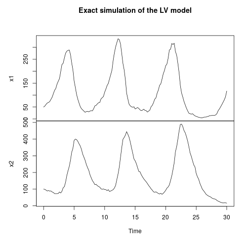
Alternatively, we can instantiate the example models using a continuous state rather than a discrete state, and then simulate using algorithms based on continous approximations, such as Euler-Maruyama simulation of a chemical Langevin equation (CLE) approximation.

val stepCle = Step.cle(SpnModels.lv[DoubleState]())
val tsCle = Sim.ts(DenseVector(50.0, 100.0), 0.0, 20.0, 0.05, stepCle)
Sim.plotTs(tsCle, "Euler-Maruyama/CLE simulation of the LV model")

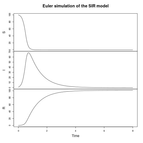
If we want to ignore noise temporarily, there’s also a simple continuous deterministic Euler integrator built-in.

val stepE = Step.euler(SpnModels.lv[DoubleState]())
val tsE = Sim.ts(DenseVector(50.0, 100.0), 0.0, 20.0, 0.05, stepE)
Sim.plotTs(tsE, "Continuous-deterministic Euler simulation of the LV model")

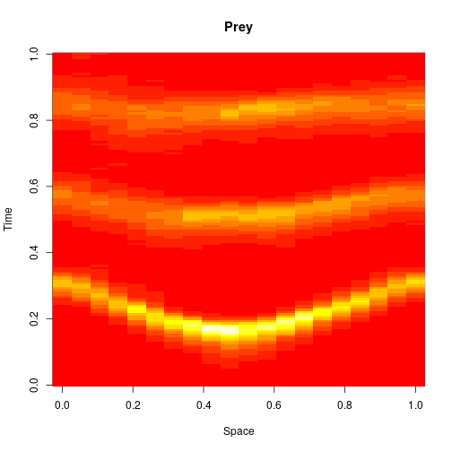
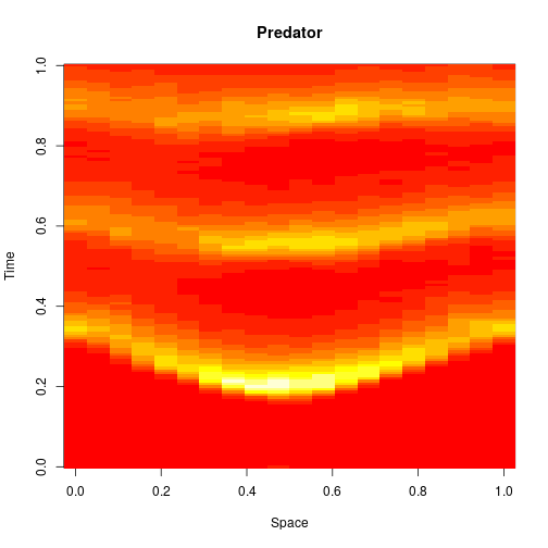
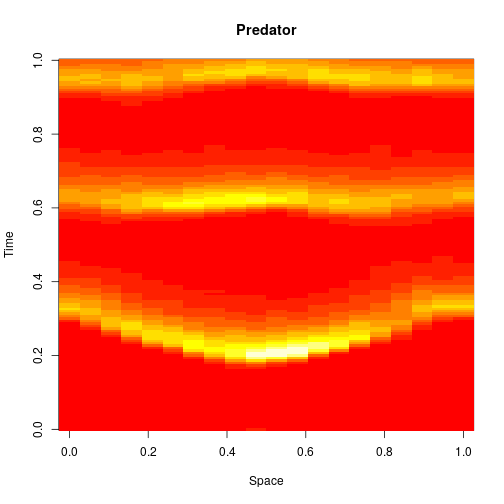
Spatial stochastic reaction-diffusion simulation

We can do 1d reaction-diffusion simulation with something like:

val N = 50; val T = 40.0
val model = SpnModels.lv[IntState]()
val step = Spatial.gillespie1d(model,DenseVector(0.8, 0.8))
val x00 = DenseVector(0, 0)
val x0 = DenseVector(50, 100)
val xx00 = Vector.fill(N)(x00)
val xx0 = xx00.updated(N/2,x0)
val output = Sim.ts(xx0, 0.0, T, 0.2, step)
Spatial.plotTs1d(output)

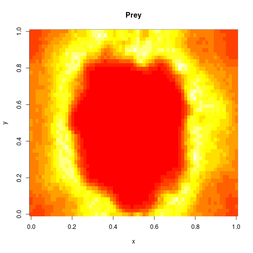
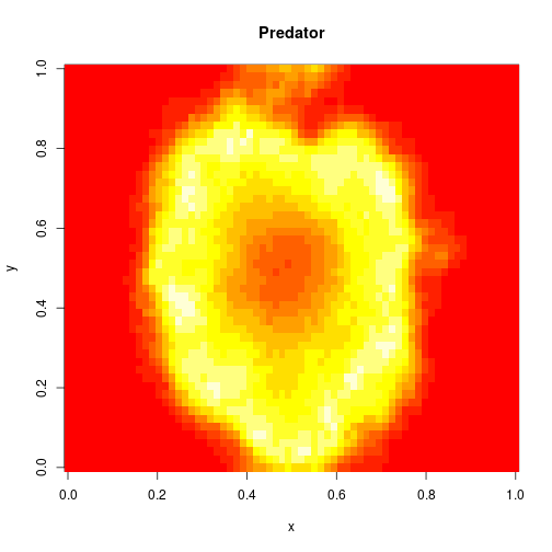
For 2d simulation, we use PMatrix, a comonadic matrix/image type defined within the library, with parallelised map and coflatMap (cobind) operations. See my post on comonads for scientific computing for further details on the concepts underpinning this, though note that it isn’t necessary to understand comonads to use the library.

val r = 20; val c = 30
val model = SpnModels.lv[DoubleState]()
val step = Spatial.cle2d(model, DenseVector(0.6, 0.6), 0.05)
val x00 = DenseVector(0.0, 0.0)
val x0 = DenseVector(50.0, 100.0)
val xx00 = PMatrix(r, c, Vector.fill(r*c)(x00))
val xx0 = xx00.updated(c/2, r/2, x0)
val output = step(xx0, 0.0, 8.0)
val f = Figure("2d LV reaction-diffusion simulation")
val p0 = f.subplot(2, 1, 0)
p0 += image(PMatrix.toBDM(output map (_.data(0))))
val p1 = f.subplot(2, 1, 1)
p1 += image(PMatrix.toBDM(output map (_.data(1))))

Bayesian parameter inference

The library also includes functions for carrying out parameter inference for stochastic dynamical systems models, using particle MCMC, ABC and ABC-SMC. See the examples directory for further details.

Next steps

Having worked through this post, the next step is to work through the tutorial. There is some overlap of content with this blog post, but the tutorial goes into more detail regarding the basics. It also finishes with suggestions for how to proceed further.

Source

This post started out as a tut document (the Scala equivalent of an RMarkdown document). The source can be found here.

The smfsb R package

Introduction

In the previous post I gave a brief introduction to the third edition of my textbook, Stochastic modelling for systems biology. The algorithms described in the book are illustrated by implementations in R. These implementations are collected together in an R package on CRAN called smfsb. This post will provide a brief introduction to the package and its capabilities.

Installation

The package is on CRAN – see the CRAN package page for details. So the simplest way to install it is to enter

install.packages("smfsb")

at the R command prompt. This will install the latest version that is on CRAN. Once installed, the package can be loaded with

library(smfsb)

The package is well-documented, so further information can be obtained with the usual R mechanisms, such as

vignette(package="smfsb")
vignette("smfsb")
help(package="smfsb")
?StepGillespie
example(StepCLE1D)

The version of the package on CRAN is almost certainly what you want. However, the package is developed on R-Forge – see the R-Forge project page for details. So the very latest version of the package can always be installed with

install.packages("smfsb", repos="http://R-Forge.R-project.org")

if you have a reason for wanting it.

A brief tutorial

The vignette gives a quick introduction the the library, which I don’t need to repeat verbatim here. If you are new to the package, I recommend working through that before continuing. Here I’ll concentrate on some of the new features associated with the third edition.

Simulating stochastic kinetic models

Much of the book is concerned with the simulation of stochastic kinetic models using exact and approximate algorithms. Although the primary focus of the text is the application to modelling of intra-cellular processes, the methods are also appropriate for population modelling of ecological and epidemic processes. For example, we can start by simulating a simple susceptible-infectious-recovered (SIR) disease epidemic model.

set.seed(2)
data(spnModels)

stepSIR = StepGillespie(SIR)
plot(simTs(SIR$M, 0, 8, 0.05, stepSIR),
  main="Exact simulation of the SIR model")

Exact simulation of the SIR epidemic model
The focus of the text is stochastic simulation of discrete models, so that is the obvious place to start. But there is also support for continuous deterministic simulation.

plot(simTs(SIR$M, 0, 8, 0.05, StepEulerSPN(SIR)),
  main="Euler simulation of the SIR model")

Euler simulation of the SIR model
My favourite toy population dynamics model is the Lotka-Volterra (LV) model, so I tend to use this frequently as a running example throughout the book. We can simulate this (exactly) as follows.

stepLV = StepGillespie(LV)
plot(simTs(LV$M, 0, 30, 0.2, stepLV),
  main="Exact simulation of the LV model")

Exact simulation of the Lotka-Volterra model

Stochastic reaction-diffusion modelling

The first two editions of the book were almost exclusively concerned with well-mixed systems, where spatial effects are ignorable. One of the main new features of the third edition is the inclusion of a new chapter on spatially extended systems. The focus is on models related to the reaction diffusion master equation (RDME) formulation, rather than individual particle-based simulations. For these models, space is typically divided into a regular grid of voxels, with reactions taking place as normal within each voxel, and additional reaction events included, corresponding to the diffusion of particles to adjacent voxels. So to specify such models, we just need an initial condition, a reaction model, and diffusion coefficients (one for each reacting species). So, we can carry out exact simulation of an RDME model for a 1D spatial domain as follows.

N=20; T=30
x0=matrix(0, nrow=2, ncol=N)
rownames(x0) = c("x1", "x2")
x0[,round(N/2)] = LV$M
stepLV1D = StepGillespie1D(LV, c(0.6, 0.6))
xx = simTs1D(x0, 0, T, 0.2, stepLV1D, verb=TRUE)
image(xx[1,,], main="Prey", xlab="Space", ylab="Time")

Discrete 1D simulation of the LV model

image(xx[2,,], main="Predator", xlab="Space", ylab="Time")

Discrete 1D simulation of the LV model
Exact simulation of discrete stochastic reaction diffusion systems is very expensive (and the reference implementation provided in the package is very inefficient), so we will often use diffusion approximations based on the CLE.

stepLV1DC = StepCLE1D(LV, c(0.6, 0.6))
xx = simTs1D(x0, 0, T, 0.2, stepLV1D)
image(xx[1,,], main="Prey", xlab="Space", ylab="Time")

Spatial CLE simulation of the 1D LV model

image(xx[2,,], main="Predator", xlab="Space", ylab="Time")

Spatial CLE simulation of the 1D LV model
We can think of this algorithm as an explicit numerical integration of the obvious SPDE approximation to the exact model.

The package also includes support for simulation of 2D systems. Again, we can use the Spatial CLE to speed things up.

m=70; n=50; T=10
data(spnModels)
x0=array(0, c(2,m,n))
dimnames(x0)[[1]]=c("x1", "x2")
x0[,round(m/2),round(n/2)] = LV$M
stepLV2D = StepCLE2D(LV, c(0.6,0.6), dt=0.05)
xx = simTs2D(x0, 0, T, 0.5, stepLV2D)
N = dim(xx)[4]
image(xx[1,,,N],main="Prey",xlab="x",ylab="y")

Spatial CLE simulation of the 2D LV model

image(xx[2,,,N],main="Predator",xlab="x",ylab="y")

Spatial CLE simulation of the 2D LV model

Bayesian parameter inference

Although much of the book is concerned with the problem of forward simulation, the final chapters are concerned with the inverse problem of estimating model parameters, such as reaction rate constants, from data. A computational Bayesian approach is adopted, with the main emphasis being placed on “likelihood free” methods, which rely on forward simulation to avoid explicit computation of sample path likelihoods. The second edition included some rudimentary code for a likelihood free particle marginal Metropolis-Hastings (PMMH) particle Markov chain Monte Carlo (pMCMC) algorithm. The third edition includes a more complete and improved implementation, in addition to approximate inference algorithms based on approximate Bayesian computation (ABC).

The key function underpinning the PMMH approach is pfMLLik, which computes an estimate of marginal model log-likelihood using a (bootstrap) particle filter. There is a new implementation of this function with the third edition. There is also a generic implementation of the Metropolis-Hastings algorithm, metropolisHastings, which can be combined with pfMLLik to create a PMMH algorithm. PMMH algorithms are very slow, but a full demo of how to use these functions for parameter inference is included in the package and can be run with

demo(PMCMC)

Simple rejection-based ABC methods are facilitated by the (very simple) function abcRun, which just samples from a prior and then carries out independent simulations in parallel before computing summary statistics. A simple illustration of the use of the function is given below.

data(LVdata)
rprior <- function() { exp(c(runif(1, -3, 3),runif(1,-8,-2),runif(1,-4,2))) }
rmodel <- function(th) { simTs(c(50,100), 0, 30, 2, stepLVc, th) }
sumStats <- identity
ssd = sumStats(LVperfect)
distance <- function(s) {
    diff = s - ssd
    sqrt(sum(diff*diff))
}
rdist <- function(th) { distance(sumStats(rmodel(th))) }
out = abcRun(10000, rprior, rdist)
q=quantile(out$dist, c(0.01, 0.05, 0.1))
print(q)
##       1%       5%      10% 
## 772.5546 845.8879 881.0573
accepted = out$param[out$dist < q[1],]
print(summary(accepted))
##        V1                V2                  V3         
##  Min.   :0.06498   Min.   :0.0004467   Min.   :0.01887  
##  1st Qu.:0.16159   1st Qu.:0.0012598   1st Qu.:0.04122  
##  Median :0.35750   Median :0.0023488   Median :0.14664  
##  Mean   :0.68565   Mean   :0.0046887   Mean   :0.36726  
##  3rd Qu.:0.86708   3rd Qu.:0.0057264   3rd Qu.:0.36870  
##  Max.   :4.76773   Max.   :0.0309364   Max.   :3.79220
print(summary(log(accepted)))
##        V1                V2               V3         
##  Min.   :-2.7337   Min.   :-7.714   Min.   :-3.9702  
##  1st Qu.:-1.8228   1st Qu.:-6.677   1st Qu.:-3.1888  
##  Median :-1.0286   Median :-6.054   Median :-1.9198  
##  Mean   :-0.8906   Mean   :-5.877   Mean   :-1.9649  
##  3rd Qu.:-0.1430   3rd Qu.:-5.163   3rd Qu.:-0.9978  
##  Max.   : 1.5619   Max.   :-3.476   Max.   : 1.3329

Naive rejection-based ABC algorithms are notoriously inefficient, so the library also includes an implementation of a more efficient, sequential version of ABC, often known as ABC-SMC, in the function abcSmc. This function requires specification of a perturbation kernel to “noise up” the particles at each algorithm sweep. Again, the implementation is parallel, using the parallel package to run the required simulations in parallel on multiple cores. A simple illustration of use is given below.

rprior <- function() { c(runif(1, -3, 3), runif(1, -8, -2), runif(1, -4, 2)) }
dprior <- function(x, ...) { dunif(x[1], -3, 3, ...) + 
    dunif(x[2], -8, -2, ...) + dunif(x[3], -4, 2, ...) }
rmodel <- function(th) { simTs(c(50,100), 0, 30, 2, stepLVc, exp(th)) }
rperturb <- function(th){th + rnorm(3, 0, 0.5)}
dperturb <- function(thNew, thOld, ...){sum(dnorm(thNew, thOld, 0.5, ...))}
sumStats <- identity
ssd = sumStats(LVperfect)
distance <- function(s) {
    diff = s - ssd
    sqrt(sum(diff*diff))
}
rdist <- function(th) { distance(sumStats(rmodel(th))) }
out = abcSmc(5000, rprior, dprior, rdist, rperturb,
    dperturb, verb=TRUE, steps=6, factor=5)
## 6 5 4 3 2 1
print(summary(out))
##        V1                V2               V3        
##  Min.   :-2.9961   Min.   :-7.988   Min.   :-3.999  
##  1st Qu.:-1.9001   1st Qu.:-6.786   1st Qu.:-3.428  
##  Median :-1.2571   Median :-6.167   Median :-2.433  
##  Mean   :-1.0789   Mean   :-6.014   Mean   :-2.196  
##  3rd Qu.:-0.2682   3rd Qu.:-5.261   3rd Qu.:-1.161  
##  Max.   : 2.1128   Max.   :-2.925   Max.   : 1.706

We can then plot some results with

hist(out[,1],30,main="log(c1)")

ABC-SMC posterior for the LV model

hist(out[,2],30,main="log(c2)")

ABC-SMC posterior for the LV model

hist(out[,3],30,main="log(c3)")

ABC-SMC posterior for the LV model

Although the inference methods are illustrated in the book in the context of parameter inference for stochastic kinetic models, their implementation is generic, and can be used with any appropriate parameter inference problem.

The smfsbSBML package

smfsbSBML is another R package associated with the third edition of the book. This package is not on CRAN due to its dependency on a package not on CRAN, and hence is slightly less straightforward to install. Follow the available installation instructions to install the package. Once installed, you should be able to load the package with

library(smfsbSBML)

This package provides a function for reading in SBML files and parsing them into the simulatable stochastic Petri net (SPN) objects used by the main smfsb R package. Examples of suitable SBML models are included in the main smfsb GitHub repo. An appropriate SBML model can be read and parsed with a command like:

model = sbml2spn("mySbmlModel.xml")

The resulting value, model is an SPN object which can be passed in to simulation functions such as StepGillespie for constructing stochastic simulation algorithms.

Other software

In addition to the above R packages, I also have some Python scripts for converting between SBML and the SBML-shorthand notation I use in the book. See the SBML-shorthand page for further details.

Although R is a convenient language for teaching and learning about stochastic simulation, it isn’t ideal for serious research-level scientific computing or computational statistics. So for the third edition of the book I have also developed scala-smfsb, a library written in the Scala programming language, which re-implements all of the models and algorithms from the third edition of the book in Scala, a fast, efficient, strongly-typed, compiled, functional programming language. I’ll give an introduction to this library in a subsequent post, but in the meantime, it is already well documented, so see the scala-smfsb repo for further details, including information on installation, getting started, a tutorial, examples, API docs, etc.

Source

This blog post started out as an RMarkdown document, the source of which can be found here.

Stochastic Modelling for Systems Biology, third edition

The third edition of my textbook, Stochastic Modelling for Systems Biology has recently been published by Chapman & Hall/CRC Press. The book has ISBN-10 113854928-2 and ISBN-13 978-113854928-9. It can be ordered from CRC Press, Amazon.com, Amazon.co.uk and similar book sellers.

I was fairly happy with the way that the second edition, published in 2011, turned out, and so I haven’t substantially re-written any of the text for the third edition. Instead, I’ve concentrated on adding in new material and improving the associated on-line resources. Those on-line resources are all free and open source, and hence available to everyone, irrespective of whether you have a copy of the new edition. I’ll give an introduction to those resources below (and in subsequent posts). The new material can be briefly summarised as follows:

  • New chapter on spatially extended systems, covering the spatial Gillespie algorithm for reaction diffusion master equation (RDME) models in 1- and 2-d, the next subvolume method, spatial CLE, scaling issues, etc.
  • Significantly expanded chapter on inference for stochastic kinetic models from data, covering approximate methods of inference (ABC), including ABC-SMC. The material relating to particle MCMC has also been improved and extended.
  • Updated R package, including code relating to all of the new material
  • New R package for parsing SBML models into simulatable stochastic Petri net models
  • New software library, written in Scala, replicating most of the functionality of the R packages in a fast, compiled, strongly typed, functional language

New content

Although some minor edits and improvements have been made throughout the text, there are two substantial new additions to the text in this new edition. The first is an entirely new chapter on spatially extended systems. The first two editions of the text focused on the implications of discreteness and stochasticity in chemical reaction systems, but maintained the well-mixed assumption throughout. This is a reasonable first approach, since discreteness and stochasticity are most pronounced in very small volumes where diffusion should be rapid. In any case, even these non-spatial models have very interesting behaviour, and become computationally challenging very quickly for non-trivial reaction networks. However, we know that, in fact, the cell is a very crowded environment, and so even at small spatial scales, many interesting processes are diffusion limited. It therefore seems appropriate to dedicate one chapter (the new Chapter 9) to studying some of the implications of relaxing the well-mixed assumption. Entire books can be written on stochastic reaction-diffusion systems, so here only a brief introduction is provided, based mainly around models in the reaction-diffusion master equation (RDME) style. Exact stochastic simulation algorithms are discussed, and implementations provided in the 1- and 2-d cases, and an appropriate Langevin approximation is examined, the spatial CLE.

The second major addition is to the chapter on inference for stochastic kinetic models from data (now Chapter 11). The second edition of the book included a discussion of “likelihood free” Bayesian MCMC methods for inference, and provided a working implementation of likelihood free particle marginal Metropolis-Hastings (PMMH) for stochastic kinetic models. The third edition improves on that implementation, and discusses approximate Bayesian computation (ABC) as an alternative to MCMC for likelihood free inference. Implementation issues are discussed, and sequential ABC approaches are examined, concentrating in particular on the method known as ABC-SMC.

New software and on-line resources

Accompanying the text are new and improved on-line resources, all well-documented, free, and open source.

New website/GitHub repo

Information and materials relating to the previous editions were kept on my University website. All materials relating to this new edition are kept in a public GitHub repo: darrenjw/smfsb. This will be simpler to maintain, and will make it much easier for people to make copies of the material for use and studying off-line.

Updated R package(s)

Along with the second edition of the book I released an accompanying R package, “smfsb”, published on CRAN. This was a very popular feature, allowing anyone with R to trivially experiment with all of the models and algorithms discussed in the text. This R package has been updated, and a new version has been published to CRAN. The updates are all backwards-compatible with the version associated with the second edition of the text, so owners of that edition can still upgrade safely. I’ll give a proper introduction to the package, including the new features, in a subsequent post, but in the meantime, you can install/upgrade the package from a running R session with

install.packages("smfsb")

and then pop up a tutorial vignette with:

vignette("smfsb")

This should be enough to get you started.

In addition to the main R package, there is an additional R package for parsing SBML models into models that can be simulated within R. This package is not on CRAN, due to its dependency on a non-CRAN package. See the repo for further details.

There are also Python scripts available for converting SBML models to and from the shorthand SBML notation used in the text.

New Scala library

Another major new resource associated with the third edition of the text is a software library written in the Scala programming language. This library provides Scala implementations of all of the algorithms discussed in the book and implemented in the associated R packages. This then provides example implementations in a fast, efficient, compiled language, and is likely to be most useful for people wanting to use the methods in the book for research. Again, I’ll provide a tutorial introduction to this library in a subsequent post, but it is well-documented, with all necessary information needed to get started available at the scala-smfsb repo/website, including a step-by-step tutorial and some additional examples.

Summary stats for ABC

Introduction

In the previous post I gave a very brief introduction to ABC, including a simple example for inferring the parameters of a Markov process given some time series observations. Towards the end of the post I observed that there were (at least!) two potential problems with scaling up the simple approach described, one relating to the dimension of the data and the other relating to the dimension of the parameter space. Before moving on to the (to me, more interesting) problem of the dimension of the parameter space, I will briefly discuss the data dimension problem in this post, and provide a couple of references for further reading.

Summary stats

Recall that the simple rejection sampling approach to ABC involves first sampling a candidate parameter \theta^\star from the prior and then sampling a corresponding data set x^\star from the model. This simulated data set is compared with the true data x using some (pseudo-)norm, \Vert\cdot\Vert, and accepting \theta^\star if the simulated data set is sufficiently close to the true data, \Vert x^\star - x\Vert <\epsilon. It should be clear that if we are using a proper norm then as \epsilon tends to zero the distribution of the accepted values tends to the desired posterior distribution of the parameters given the data.

However, smaller choices of \epsilon will lead to higher rejection rates. This will be a particular problem in the context of high-dimensional x, where it is often unrealistic to expect a close match between all components of x and the simulated data x^\star, even for a good choice of \theta^\star. In this case, it makes more sense to look for good agreement between particular aspects of x, such as the mean, or variance, or auto-correlation, depending on the exact problem and context. If we can find a finite set of sufficient statistics, s(x) for \theta, then it should be clear that replacing the acceptance criterion with \Vert s(x^\star) - s(x)\Vert <\epsilon will also lead to a scheme tending to the true posterior as \epsilon tends to zero (assuming a proper norm on the space of sufficient statistics), and will typically be better than the naive method, since the sufficient statistics will be of lower dimension and less “noisy” that the raw data, leading to higher acceptance rates with no loss of information.

Unfortunately for most problems of practical interest it is not possible to find low-dimensional sufficient statistics, and so people in practice use domain knowledge and heuristics to come up with a set of summary statistics, s(x) which they hope will closely approximate sufficient statistics. There is still a question as to how these statistics should be weighted or transformed to give a particular norm. This can be done using theory or heuristics, and some relevant references for this problem are given at the end of the post.

Implementation in R

Let’s now look at the problem from the previous post. Here, instead of directly computing the Euclidean distance between the real and simulated data, we will look at the Euclidean distance between some (normalised) summary statistics. First we will load some packages and set some parameters.

require(smfsb)
require(parallel)
options(mc.cores=4)
data(LVdata)
 
N=1e7
bs=1e5
batches=N/bs
message(paste("N =",N," | bs =",bs," | batches =",batches))

Next we will define some summary stats for a univariate time series – the mean, the (log) variance, and the first two auto-correlations.

ssinit <- function(vec)
{
  ac23=as.vector(acf(vec,lag.max=2,plot=FALSE)$acf)[2:3]
  c(mean(vec),log(var(vec)+1),ac23)
}

Once we have this, we can define some stats for a bivariate time series by combining the stats for the two component series, along with the cross-correlation between them.

ssi <- function(ts)
{
  c(ssinit(ts[,1]),ssinit(ts[,2]),cor(ts[,1],ts[,2]))
}

This gives a set of summary stats, but these individual statistics are potentially on very different scales. They can be transformed and re-weighted in a variety of ways, usually on the basis of a pilot run which gives some information about the distribution of the summary stats. Here we will do the simplest possible thing, which is to normalise the variance of the stats on the basis of a pilot run. This is not at all optimal – see the references at the end of the post for a description of better methods.

message("Batch 0: Pilot run batch")
prior=cbind(th1=exp(runif(bs,-6,2)),th2=exp(runif(bs,-6,2)),th3=exp(runif(bs,-6,2)))
rows=lapply(1:bs,function(i){prior[i,]})
samples=mclapply(rows,function(th){simTs(c(50,100),0,30,2,stepLVc,th)})
sumstats=mclapply(samples,ssi)
sds=apply(sapply(sumstats,c),1,sd)
print(sds)

# now define a standardised distance
ss<-function(ts)
{
  ssi(ts)/sds
}

ss0=ss(LVperfect)

distance <- function(ts)
{
  diff=ss(ts)-ss0
  sum(diff*diff)
}

Now we have a normalised distance function defined, we can proceed exactly as before to obtain an ABC posterior via rejection sampling.

post=NULL
for (i in 1:batches) {
  message(paste("batch",i,"of",batches))
  prior=cbind(th1=exp(runif(bs,-6,2)),th2=exp(runif(bs,-6,2)),th3=exp(runif(bs,-6,2)))
  rows=lapply(1:bs,function(i){prior[i,]})
  samples=mclapply(rows,function(th){simTs(c(50,100),0,30,2,stepLVc,th)})
  dist=mclapply(samples,distance)
  dist=sapply(dist,c)
  cutoff=quantile(dist,1000/N,na.rm=TRUE)
  post=rbind(post,prior[dist<cutoff,])
}
message(paste("Finished. Kept",dim(post)[1],"simulations"))

Having obtained the posterior, we can use the following code to plot the results.

th=c(th1 = 1, th2 = 0.005, th3 = 0.6)
op=par(mfrow=c(2,3))
for (i in 1:3) {
  hist(post[,i],30,col=5,main=paste("Posterior for theta[",i,"]",sep=""))
  abline(v=th[i],lwd=2,col=2)
}
for (i in 1:3) {
  hist(log(post[,i]),30,col=5,main=paste("Posterior for log(theta[",i,"])",sep=""))
  abline(v=log(th[i]),lwd=2,col=2)
}
par(op)

This gives the plot shown below. From this we can see that the ABC posterior obtained here is very similar to that obtained in the previous post using the full data. Here the dimension reduction is not that great – reducing from 32 data points to 9 summary statistics – and so the improvement in performance is not that noticable. But in higher dimensional problems reducing the dimension of the data is practically essential.

ABC Posterior

Summary and References

As before, I recommend the wikipedia article on approximate Bayesian computation for further information and a comprehensive set of references for further reading. Here I just want to highlight two references particularly relevant to the issue of summary statistics. It is quite difficult to give much practical advice on how to construct good summary statistics, but how to transform a set of summary stats in a “good” way is a problem that is reasonably well understood. In this post I did something rather naive (normalising the variance), but the following two papers describe much better approaches.

I still haven’t addressed the issue of a high-dimensional parameter space – that will be the topic of a subsequent post.

The complete R script

require(smfsb)
require(parallel)
options(mc.cores=4)
data(LVdata)
 
N=1e6
bs=1e5
batches=N/bs
message(paste("N =",N," | bs =",bs," | batches =",batches))
 
ssinit <- function(vec)
{
  ac23=as.vector(acf(vec,lag.max=2,plot=FALSE)$acf)[2:3]
  c(mean(vec),log(var(vec)+1),ac23)
}

ssi <- function(ts)
{
  c(ssinit(ts[,1]),ssinit(ts[,2]),cor(ts[,1],ts[,2]))
}

message("Batch 0: Pilot run batch")
prior=cbind(th1=exp(runif(bs,-6,2)),th2=exp(runif(bs,-6,2)),th3=exp(runif(bs,-6,2)))
rows=lapply(1:bs,function(i){prior[i,]})
samples=mclapply(rows,function(th){simTs(c(50,100),0,30,2,stepLVc,th)})
sumstats=mclapply(samples,ssi)
sds=apply(sapply(sumstats,c),1,sd)
print(sds)

# now define a standardised distance
ss<-function(ts)
{
  ssi(ts)/sds
}

ss0=ss(LVperfect)

distance <- function(ts)
{
  diff=ss(ts)-ss0
  sum(diff*diff)
}

post=NULL
for (i in 1:batches) {
  message(paste("batch",i,"of",batches))
  prior=cbind(th1=exp(runif(bs,-6,2)),th2=exp(runif(bs,-6,2)),th3=exp(runif(bs,-6,2)))
  rows=lapply(1:bs,function(i){prior[i,]})
  samples=mclapply(rows,function(th){simTs(c(50,100),0,30,2,stepLVc,th)})
  dist=mclapply(samples,distance)
  dist=sapply(dist,c)
  cutoff=quantile(dist,1000/N,na.rm=TRUE)
  post=rbind(post,prior[dist<cutoff,])
}
message(paste("Finished. Kept",dim(post)[1],"simulations"))

# plot the results
th=c(th1 = 1, th2 = 0.005, th3 = 0.6)
op=par(mfrow=c(2,3))
for (i in 1:3) {
  hist(post[,i],30,col=5,main=paste("Posterior for theta[",i,"]",sep=""))
  abline(v=th[i],lwd=2,col=2)
}
for (i in 1:3) {
  hist(log(post[,i]),30,col=5,main=paste("Posterior for log(theta[",i,"])",sep=""))
  abline(v=log(th[i]),lwd=2,col=2)
}
par(op)

Introduction to Approximate Bayesian Computation (ABC)

Many of the posts in this blog have been concerned with using MCMC based methods for Bayesian inference. These methods are typically “exact” in the sense that they have the exact posterior distribution of interest as their target equilibrium distribution, but are obviously “approximate”, in that for any finite amount of computing time, we can only generate a finite sample of correlated realisations from a Markov chain that we hope is close to equilibrium.

Approximate Bayesian Computation (ABC) methods go a step further, and generate samples from a distribution which is not the true posterior distribution of interest, but a distribution which is hoped to be close to the real posterior distribution of interest. There are many variants on ABC, and I won’t get around to explaining all of them in this blog. The wikipedia page on ABC is a good starting point for further reading. In this post I’ll explain the most basic rejection sampling version of ABC, and in a subsequent post, I’ll explain a sequential refinement, often referred to as ABC-SMC. As usual, I’ll use R code to illustrate the ideas.

Basic idea

There is a close connection between “likelihood free” MCMC methods and those of approximate Bayesian computation (ABC). To keep things simple, consider the case of a perfectly observed system, so that there is no latent variable layer. Then there are model parameters \theta described by a prior \pi(\theta), and a forwards-simulation model for the data x, defined by \pi(x|\theta). It is clear that a simple algorithm for simulating from the desired posterior \pi(\theta|x) can be obtained as follows. First simulate from the joint distribution \pi(\theta,x) by simulating \theta^\star\sim\pi(\theta) and then x^\star\sim \pi(x|\theta^\star). This gives a sample (\theta^\star,x^\star) from the joint distribution. A simple rejection algorithm which rejects the proposed pair unless x^\star matches the true data x clearly gives a sample from the required posterior distribution.

Exact rejection sampling

  • 1. Sample \theta^\star \sim \pi(\theta^\star)
  • 2. Sample x^\star\sim \pi(x^\star|\theta^\star)
  • 3. If x^\star=x, keep \theta^\star as a sample from \pi(\theta|x), otherwise reject.
  • 4. Return to step 1.

This algorithm is exact, and for discrete x will have a non-zero acceptance rate. However, in most interesting problems the rejection rate will be intolerably high. In particular, the acceptance rate will typically be zero for continuous valued x.

ABC rejection sampling

The ABC “approximation” is to accept values provided that x^\star is “sufficiently close” to x. In the first instance, we can formulate this as follows.

  • 1. Sample \theta^\star \sim \pi(\theta^\star)
  • 2. Sample x^\star\sim \pi(x^\star|\theta^\star)
  • 3. If \Vert x^\star-x\Vert< \epsilon, keep \theta^\star as a sample from \pi(\theta|x), otherwise reject.
  • 4. Return to step 1.

Euclidean distance is usually chosen as the norm, though any norm can be used. This procedure is “honest”, in the sense that it produces exact realisations from

\theta^\star\big|\Vert x^\star-x\Vert < \epsilon.

For suitable small choice of \epsilon, this will closely approximate the true posterior. However, smaller choices of \epsilon will lead to higher rejection rates. This will be a particular problem in the context of high-dimensional x, where it is often unrealistic to expect a close match between all components of x and the simulated data x^\star, even for a good choice of \theta^\star. In this case, it makes more sense to look for good agreement between particular aspects of x, such as the mean, or variance, or auto-correlation, depending on the exact problem and context.

In the simplest case, this is done by forming a (vector of) summary statistic(s), s(x^\star) (ideally a sufficient statistic), and accepting provided that \Vert s(x^\star)-s(x)\Vert<\epsilon for some suitable choice of metric and \epsilon. We will return to this issue in a subsequent post.

Inference for an intractable Markov process

I’ll illustrate ABC in the context of parameter inference for a Markov process with an intractable transition kernel: the discrete stochastic Lotka-Volterra model. A function for simulating exact realisations from the intractable kernel is included in the smfsb CRAN package discussed in a previous post. Using pMCMC to solve the parameter inference problem is discussed in another post. It may be helpful to skim through those posts quickly to become familiar with this problem before proceeding.

So, for a given proposed set of parameters, realisations from the process can be sampled using the functions simTs and stepLV (from the smfsb package). We will use the sample data set LVperfect (from the LVdata dataset) as our “true”, or “target” data, and try to find parameters for the process which are consistent with this data. A fairly minimal R script for this problem is given below.

require(smfsb)
data(LVdata)

N=1e5
message(paste("N =",N))
prior=cbind(th1=exp(runif(N,-6,2)),th2=exp(runif(N,-6,2)),th3=exp(runif(N,-6,2)))
rows=lapply(1:N,function(i){prior[i,]})
message("starting simulation")
samples=lapply(rows,function(th){simTs(c(50,100),0,30,2,stepLVc,th)})
message("finished simulation")

distance<-function(ts)
{
  diff=ts-LVperfect
  sum(diff*diff)
}

message("computing distances")
dist=lapply(samples,distance)
message("distances computed")

dist=sapply(dist,c)
cutoff=quantile(dist,1000/N)
post=prior[dist<cutoff,]

op=par(mfrow=c(2,3))
apply(post,2,hist,30)
apply(log(post),2,hist,30)
par(op)

This script should take 5-10 minutes to run on a decent laptop, and will result in histograms of the posterior marginals for the components of \theta and \log(\theta). Note that I have deliberately adopted a functional programming style, making use of the lapply function for the most computationally intensive steps. The reason for this will soon become apparent. Note that rather than pre-specifying a cutoff \epsilon, I’ve instead picked a quantile of the distance distribution. This is common practice in scenarios where the distance is difficult to have good intuition about. In fact here I’ve gone a step further and chosen a quantile to give a final sample of size 1000. Obviously then in this case I could have just selected out the top 1000 directly, but I wanted to illustrate the quantile based approach.

One problem with the above script is that all proposed samples are stored in memory at once. This is problematic for problems involving large numbers of samples. However, it is convenient to do simulations in large batches, both for computation of quantiles, and also for efficient parallelisation. The script below illustrates how to implement a batch parallelisation strategy for this problem. Samples are generated in batches of size 10^4, and only the best fitting samples are stored before the next batch is processed. This strategy can be used to get a good sized sample based on a more stringent acceptance criterion at the cost of addition simulation time. Note that the parallelisation code will only work with recent versions of R, and works by replacing calls to lapply with the parallel version, mclapply. You should notice an appreciable speed-up on a multicore machine.

require(smfsb)
require(parallel)
options(mc.cores=4)
data(LVdata)

N=1e5
bs=1e4
batches=N/bs
message(paste("N =",N," | bs =",bs," | batches =",batches))

distance<-function(ts)
{
  diff=ts[,1]-LVprey
  sum(diff*diff)
}

post=NULL
for (i in 1:batches) {
  message(paste("batch",i,"of",batches))
  prior=cbind(th1=exp(runif(bs,-6,2)),th2=exp(runif(bs,-6,2)),th3=exp(runif(bs,-6,2)))
  rows=lapply(1:bs,function(i){prior[i,]})
  samples=mclapply(rows,function(th){simTs(c(50,100),0,30,2,stepLVc,th)})
  dist=mclapply(samples,distance)
  dist=sapply(dist,c)
  cutoff=quantile(dist,1000/N)
  post=rbind(post,prior[dist<cutoff,])
}
message(paste("Finished. Kept",dim(post)[1],"simulations"))

op=par(mfrow=c(2,3))
apply(post,2,hist,30)
apply(log(post),2,hist,30)
par(op)

Note that there is an additional approximation here, since the top 100 samples from each of 10 batches of simulations won’t correspond exactly to the top 1000 samples overall, but given all of the other approximations going on in ABC, this one is likely to be the least of your worries.

Now, if you compare the approximate posteriors obtained here with the “true” posteriors obtained in an earlier post using pMCMC, you will see that these posteriors are really quite poor. However, this isn’t a very fair comparison, since we’ve only done 10^5 simulations. Jacking N up to 10^7 gives the ABC posterior below.

ABC posterior from 10^7 iterations
ABC posterior from 10^7 samples

This is a bit better, but really not great. There are two basic problems with the simplistic ABC strategy adopted here, one related to the dimensionality of the data and the other the dimensionality of the parameter space. The most basic problem that we have here is the dimensionality of the data. We have 16 (bivariate) observations, so we want our stochastic simulation to shoot at a point in a 16- or 32-dimensional space. That’s a tough call. The standard way to address this problem is to reduce the dimension of the data by introducing a few carefully chosen summary statistics and then just attempting to hit those. I’ll illustrate this in a subsequent post. The other problem is that often the prior and posterior over the parameters are quite different, and this problem too is exacerbated as the dimension of the parameter space increases. The standard way to deal with this is to sequentially adapt from the prior through a sequence of ABC posteriors. I’ll examine this in a future post as well, once I’ve also posted an introduction to the use of sequential Monte Carlo (SMC) samplers for static problems.

Further reading

For further reading, I suggest browsing the reference list of the Wikipedia page for ABC. Also look through the list of software on that page. In particular, note that there is a CRAN package, abc, providing R support for ABC. There is a vignette for this package which should be sufficient to get started.