The scala-smfsb library

In the previous post I gave a very quick introduction to the smfsb R package. As mentioned in that post, although good for teaching and learning, R isn’t a great language for serious scientific computing or computational statistics. So for the publication of the third edition of my textbook, Stochastic modelling for systems biology, I have created a library in the Scala programming language replicating the functionality provided by the R package. Here I will give a very quick introduction to the scala-smfsb library. Some familiarity with both Scala and the smfsb R package will be helpful, but is not strictly necessary. Note that the library relies on the Scala Breeze library for linear algebra and probability distributions, so some familiarity with that library can also be helpful.

Setup

To follow the along you need to have Sbt installed, and this in turn requires a recent JDK. If you are new to Scala, you may find the setup page for my Scala course to be useful, but note that on many Linux systems it can be as simple as installing the packages openjdk-8-jdk and sbt.

Once you have Sbt installed, you should be able to run it by entering sbt at your OS command line. You now need to use Sbt to create a Scala REPL with a dependency on the scala-smfsb library. There are many ways to do this, but if you are new to Scala, the simplest way is probably to start up Sbt from an empty or temporary directory (which doesn’t contain any Scala code), and then paste the following into the Sbt prompt:

set libraryDependencies += "com.github.darrenjw" %% "scala-smfsb" % "0.6"
set libraryDependencies += "org.scalanlp" %% "breeze-viz" % "0.13.2"
set scalaVersion := "2.12.6"
set scalacOptions += "-Yrepl-class-based"
console

The first time you run this it will take a little while to download and cache various library dependencies. But everything is cached, so it should be much quicker in future. When it is finished, you should have a Scala REPL ready to enter Scala code.

An introduction to scala-smfsb

It should be possible to type or copy-and-paste the commands below one-at-a-time into the Scala REPL. We need to start with a few imports.

import smfsb._
import breeze.linalg.{Vector => BVec, _}
import breeze.numerics._
import breeze.plot._

Note that I’ve renamed Breeze’s Vector type to BVec to avoid clashing with that in the Scala standard library. We are now ready to go.

Simulating models

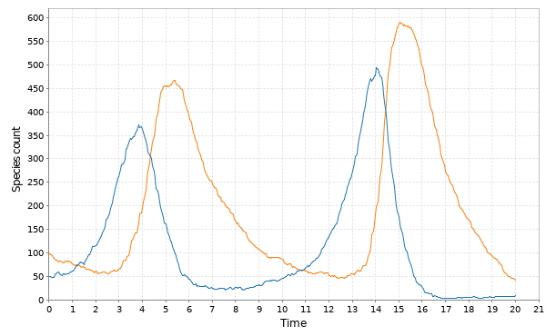
Let’s begin by instantiating a Lotka-Volterra model, simulating a single realisation of the process, and then plotting it.

// Simulate LV with Gillespie
val model = SpnModels.lv[IntState]()
val step = Step.gillespie(model)
val ts = Sim.ts(DenseVector(50, 100), 0.0, 20.0, 0.05, step)
Sim.plotTs(ts, "Gillespie simulation of LV model with default parameters")

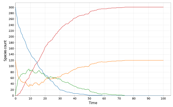
The library comes with a few other models. There’s a Michaelis-Menten enzyme kinetics model:

// Simulate other models with Gillespie
val stepMM = Step.gillespie(SpnModels.mm[IntState]())
val tsMM = Sim.ts(DenseVector(301,120,0,0), 0.0, 100.0, 0.5, stepMM)
Sim.plotTs(tsMM, "Gillespie simulation of the MM model")

and an auto-regulatory genetic network model, for example.

val stepAR = Step.gillespie(SpnModels.ar[IntState]())
val tsAR = Sim.ts(DenseVector(10, 0, 0, 0, 0), 0.0, 500.0, 0.5, stepAR)
Sim.plotTs(tsAR, "Gillespie simulation of the AR model")

If you know the book and/or the R package, these models should all be familiar.
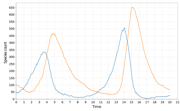
We are not restricted to exact stochastic simulation using the Gillespie algorithm. We can use an approximate Poisson time-stepping algorithm.

// Simulate LV with other algorithms
val stepPts = Step.pts(model)
val tsPts = Sim.ts(DenseVector(50, 100), 0.0, 20.0, 0.05, stepPts)
Sim.plotTs(tsPts, "Poisson time-step simulation of the LV model")

Alternatively, we can instantiate the example models using a continuous state rather than a discrete state, and then simulate using algorithms based on continous approximations, such as Euler-Maruyama simulation of a chemical Langevin equation (CLE) approximation.

val stepCle = Step.cle(SpnModels.lv[DoubleState]())
val tsCle = Sim.ts(DenseVector(50.0, 100.0), 0.0, 20.0, 0.05, stepCle)
Sim.plotTs(tsCle, "Euler-Maruyama/CLE simulation of the LV model")

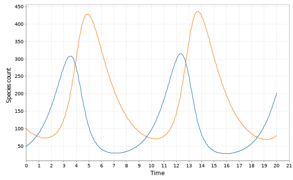
If we want to ignore noise temporarily, there’s also a simple continuous deterministic Euler integrator built-in.

val stepE = Step.euler(SpnModels.lv[DoubleState]())
val tsE = Sim.ts(DenseVector(50.0, 100.0), 0.0, 20.0, 0.05, stepE)
Sim.plotTs(tsE, "Continuous-deterministic Euler simulation of the LV model")

Spatial stochastic reaction-diffusion simulation

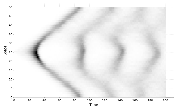
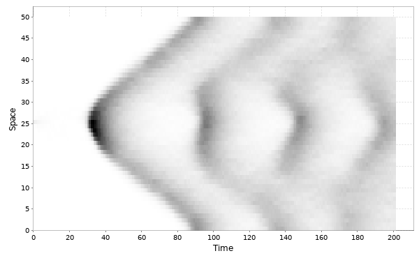
We can do 1d reaction-diffusion simulation with something like:

val N = 50; val T = 40.0
val model = SpnModels.lv[IntState]()
val step = Spatial.gillespie1d(model,DenseVector(0.8, 0.8))
val x00 = DenseVector(0, 0)
val x0 = DenseVector(50, 100)
val xx00 = Vector.fill(N)(x00)
val xx0 = xx00.updated(N/2,x0)
val output = Sim.ts(xx0, 0.0, T, 0.2, step)
Spatial.plotTs1d(output)

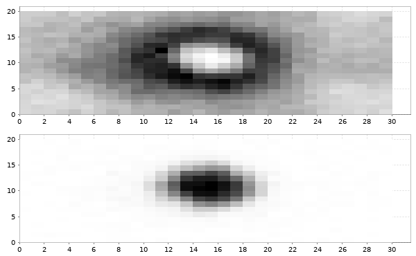
For 2d simulation, we use PMatrix, a comonadic matrix/image type defined within the library, with parallelised map and coflatMap (cobind) operations. See my post on comonads for scientific computing for further details on the concepts underpinning this, though note that it isn’t necessary to understand comonads to use the library.

val r = 20; val c = 30
val model = SpnModels.lv[DoubleState]()
val step = Spatial.cle2d(model, DenseVector(0.6, 0.6), 0.05)
val x00 = DenseVector(0.0, 0.0)
val x0 = DenseVector(50.0, 100.0)
val xx00 = PMatrix(r, c, Vector.fill(r*c)(x00))
val xx0 = xx00.updated(c/2, r/2, x0)
val output = step(xx0, 0.0, 8.0)
val f = Figure("2d LV reaction-diffusion simulation")
val p0 = f.subplot(2, 1, 0)
p0 += image(PMatrix.toBDM(output map (_.data(0))))
val p1 = f.subplot(2, 1, 1)
p1 += image(PMatrix.toBDM(output map (_.data(1))))

Bayesian parameter inference

The library also includes functions for carrying out parameter inference for stochastic dynamical systems models, using particle MCMC, ABC and ABC-SMC. See the examples directory for further details.

Next steps

Having worked through this post, the next step is to work through the tutorial. There is some overlap of content with this blog post, but the tutorial goes into more detail regarding the basics. It also finishes with suggestions for how to proceed further.

Source

This post started out as a tut document (the Scala equivalent of an RMarkdown document). The source can be found here.

Stochastic Modelling for Systems Biology, third edition

The third edition of my textbook, Stochastic Modelling for Systems Biology has recently been published by Chapman & Hall/CRC Press. The book has ISBN-10 113854928-2 and ISBN-13 978-113854928-9. It can be ordered from CRC Press, Amazon.com, Amazon.co.uk and similar book sellers.

I was fairly happy with the way that the second edition, published in 2011, turned out, and so I haven’t substantially re-written any of the text for the third edition. Instead, I’ve concentrated on adding in new material and improving the associated on-line resources. Those on-line resources are all free and open source, and hence available to everyone, irrespective of whether you have a copy of the new edition. I’ll give an introduction to those resources below (and in subsequent posts). The new material can be briefly summarised as follows:

• New chapter on spatially extended systems, covering the spatial Gillespie algorithm for reaction diffusion master equation (RDME) models in 1- and 2-d, the next subvolume method, spatial CLE, scaling issues, etc.
• Significantly expanded chapter on inference for stochastic kinetic models from data, covering approximate methods of inference (ABC), including ABC-SMC. The material relating to particle MCMC has also been improved and extended.
• Updated R package, including code relating to all of the new material
• New R package for parsing SBML models into simulatable stochastic Petri net models
• New software library, written in Scala, replicating most of the functionality of the R packages in a fast, compiled, strongly typed, functional language

New content

Although some minor edits and improvements have been made throughout the text, there are two substantial new additions to the text in this new edition. The first is an entirely new chapter on spatially extended systems. The first two editions of the text focused on the implications of discreteness and stochasticity in chemical reaction systems, but maintained the well-mixed assumption throughout. This is a reasonable first approach, since discreteness and stochasticity are most pronounced in very small volumes where diffusion should be rapid. In any case, even these non-spatial models have very interesting behaviour, and become computationally challenging very quickly for non-trivial reaction networks. However, we know that, in fact, the cell is a very crowded environment, and so even at small spatial scales, many interesting processes are diffusion limited. It therefore seems appropriate to dedicate one chapter (the new Chapter 9) to studying some of the implications of relaxing the well-mixed assumption. Entire books can be written on stochastic reaction-diffusion systems, so here only a brief introduction is provided, based mainly around models in the reaction-diffusion master equation (RDME) style. Exact stochastic simulation algorithms are discussed, and implementations provided in the 1- and 2-d cases, and an appropriate Langevin approximation is examined, the spatial CLE.

The second major addition is to the chapter on inference for stochastic kinetic models from data (now Chapter 11). The second edition of the book included a discussion of “likelihood free” Bayesian MCMC methods for inference, and provided a working implementation of likelihood free particle marginal Metropolis-Hastings (PMMH) for stochastic kinetic models. The third edition improves on that implementation, and discusses approximate Bayesian computation (ABC) as an alternative to MCMC for likelihood free inference. Implementation issues are discussed, and sequential ABC approaches are examined, concentrating in particular on the method known as ABC-SMC.

New software and on-line resources

Accompanying the text are new and improved on-line resources, all well-documented, free, and open source.

New website/GitHub repo

Information and materials relating to the previous editions were kept on my University website. All materials relating to this new edition are kept in a public GitHub repo: darrenjw/smfsb. This will be simpler to maintain, and will make it much easier for people to make copies of the material for use and studying off-line.

Updated R package(s)

Along with the second edition of the book I released an accompanying R package, “smfsb”, published on CRAN. This was a very popular feature, allowing anyone with R to trivially experiment with all of the models and algorithms discussed in the text. This R package has been updated, and a new version has been published to CRAN. The updates are all backwards-compatible with the version associated with the second edition of the text, so owners of that edition can still upgrade safely. I’ll give a proper introduction to the package, including the new features, in a subsequent post, but in the meantime, you can install/upgrade the package from a running R session with

install.packages("smfsb")

and then pop up a tutorial vignette with:

vignette("smfsb")

This should be enough to get you started.

In addition to the main R package, there is an additional R package for parsing SBML models into models that can be simulated within R. This package is not on CRAN, due to its dependency on a non-CRAN package. See the repo for further details.

There are also Python scripts available for converting SBML models to and from the shorthand SBML notation used in the text.

New Scala library

Another major new resource associated with the third edition of the text is a software library written in the Scala programming language. This library provides Scala implementations of all of the algorithms discussed in the book and implemented in the associated R packages. This then provides example implementations in a fast, efficient, compiled language, and is likely to be most useful for people wanting to use the methods in the book for research. Again, I’ll provide a tutorial introduction to this library in a subsequent post, but it is well-documented, with all necessary information needed to get started available at the scala-smfsb repo/website, including a step-by-step tutorial and some additional examples.