Introduction
This weekend I’ve been preparing some material for my upcoming Scala for statistical computing short course. As part of the course, I thought it would be useful to walk through how to think about and structure MCMC codes, and in particular, how to think about MCMC algorithms as infinite streams of state. This material is reasonably stand-alone, so it seems suitable for a blog post. Complete runnable code for the examples in this post are available from my blog repo.
A simple MH sampler
For this post I will just consider a trivial toy Metropolis algorithm using a Uniform random walk proposal to target a standard normal distribution. I’ve considered this problem before on my blog, so if you aren’t very familiar with Metropolis-Hastings algorithms, you might want to quickly review my post on Metropolis-Hastings MCMC algorithms in R before continuing. At the end of that post, I gave the following R code for the Metropolis sampler:
metrop3<-function(n=1000,eps=0.5)
{
        vec=vector("numeric", n)
        x=0
        oldll=dnorm(x,log=TRUE)
        vec[1]=x
        for (i in 2:n) {
                can=x+runif(1,-eps,eps)
                loglik=dnorm(can,log=TRUE)
                loga=loglik-oldll
                if (log(runif(1)) < loga) {
                        x=can
                        oldll=loglik
                        }
                vec[i]=x
        }
        vec
}
I will begin this post with a fairly direct translation of this algorithm into Scala:
def metrop1(n: Int = 1000, eps: Double = 0.5): DenseVector[Double] = {
    val vec = DenseVector.fill(n)(0.0)
    var x = 0.0
    var oldll = Gaussian(0.0, 1.0).logPdf(x)
    vec(0) = x
    (1 until n).foreach { i =>
      val can = x + Uniform(-eps, eps).draw
      val loglik = Gaussian(0.0, 1.0).logPdf(can)
      val loga = loglik - oldll
      if (math.log(Uniform(0.0, 1.0).draw) < loga) {
        x = can
        oldll = loglik
      }
      vec(i) = x
    }
    vec
}
This code works, and is reasonably fast and efficient, but there are several issues with it from a functional programmers perspective. One issue is that we have committed to storing all MCMC output in RAM in a DenseVector. This probably isn’t an issue here, but for some big problems we might prefer to not store the full set of states, but to just print the states to (say) the console, for possible re-direction to a file. It is easy enough to modify the code to do this:
def metrop2(n: Int = 1000, eps: Double = 0.5): Unit = {
    var x = 0.0
    var oldll = Gaussian(0.0, 1.0).logPdf(x)
    (1 to n).foreach { i =>
      val can = x + Uniform(-eps, eps).draw
      val loglik = Gaussian(0.0, 1.0).logPdf(can)
      val loga = loglik - oldll
      if (math.log(Uniform(0.0, 1.0).draw) < loga) {
        x = can
        oldll = loglik
      }
      println(x)
    }
}
But now we have two version of the algorithm. One for storing results locally, and one for streaming results to the console. This is clearly unsatisfactory, but we shall return to this issue shortly. Another issue that will jump out at functional programmers is the reliance on mutable variables for storing the state and old likelihood. Let’s fix that now by re-writing the algorithm as a tail-recursion.
@tailrec
def metrop3(n: Int = 1000, eps: Double = 0.5, x: Double = 0.0, oldll: Double = Double.MinValue): Unit = {
    if (n > 0) {
      println(x)
      val can = x + Uniform(-eps, eps).draw
      val loglik = Gaussian(0.0, 1.0).logPdf(can)
      val loga = loglik - oldll
      if (math.log(Uniform(0.0, 1.0).draw) < loga)
        metrop3(n - 1, eps, can, loglik)
      else
        metrop3(n - 1, eps, x, oldll)
    }
  }
This has eliminated the vars, and is just as fast and efficient as the previous version of the code. Note that the @tailrec annotation is optional – it just signals to the compiler that we want it to throw an error if for some reason it cannot eliminate the tail call. However, this is for the print-to-console version of the code. What if we actually want to keep the iterations in RAM for subsequent analysis? We can keep the values in an accumulator, as follows.
@tailrec
def metrop4(n: Int = 1000, eps: Double = 0.5, x: Double = 0.0, oldll: Double = Double.MinValue, acc: List[Double] = Nil): DenseVector[Double] = {
    if (n == 0)
      DenseVector(acc.reverse.toArray)
    else {
      val can = x + Uniform(-eps, eps).draw
      val loglik = Gaussian(0.0, 1.0).logPdf(can)
      val loga = loglik - oldll
      if (math.log(Uniform(0.0, 1.0).draw) < loga)
        metrop4(n - 1, eps, can, loglik, can :: acc)
      else
        metrop4(n - 1, eps, x, oldll, x :: acc)
    }
}
Factoring out the updating logic
This is all fine, but we haven’t yet addressed the issue of having different versions of the code depending on what we want to do with the output. The problem is that we have tied up the logic of advancing the Markov chain with what to do with the output. What we need to do is separate out the code for advancing the state. We can do this by defining a new function.
def newState(x: Double, oldll: Double, eps: Double): (Double, Double) = {
    val can = x + Uniform(-eps, eps).draw
    val loglik = Gaussian(0.0, 1.0).logPdf(can)
    val loga = loglik - oldll
    if (math.log(Uniform(0.0, 1.0).draw) < loga) (can, loglik) else (x, oldll)
}
This function takes as input a current state and associated log likelihood and returns a new state and log likelihood following the execution of one step of a MH algorithm. This separates the concern of state updating from the rest of the code. So now if we want to write code that prints the state, we can write it as
  @tailrec
  def metrop5(n: Int = 1000, eps: Double = 0.5, x: Double = 0.0, oldll: Double = Double.MinValue): Unit = {
    if (n > 0) {
      println(x)
      val ns = newState(x, oldll, eps)
      metrop5(n - 1, eps, ns._1, ns._2)
    }
  }
and if we want to accumulate the set of states visited, we can write that as
  @tailrec
  def metrop6(n: Int = 1000, eps: Double = 0.5, x: Double = 0.0, oldll: Double = Double.MinValue, acc: List[Double] = Nil): DenseVector[Double] = {
    if (n == 0) DenseVector(acc.reverse.toArray) else {
      val ns = newState(x, oldll, eps)
      metrop6(n - 1, eps, ns._1, ns._2, ns._1 :: acc)
    }
  }
Both of these functions call newState to do the real work, and concentrate on what to do with the sequence of states. However, both of these functions repeat the logic of how to iterate over the sequence of states.
MCMC as a stream
Ideally we would like to abstract out the details of how to do state iteration from the code as well. Most functional languages have some concept of a Stream, which represents a (potentially infinite) sequence of states. The Stream can embody the logic of how to perform state iteration, allowing us to abstract that away from our code, as well.
To do this, we will restructure our code slightly so that it more clearly maps old state to new state.
def nextState(eps: Double)(state: (Double, Double)): (Double, Double) = {
    val x = state._1
    val oldll = state._2
    val can = x + Uniform(-eps, eps).draw
    val loglik = Gaussian(0.0, 1.0).logPdf(can)
    val loga = loglik - oldll
    if (math.log(Uniform(0.0, 1.0).draw) < loga) (can, loglik) else (x, oldll)
}
The "real" state of the chain is just x, but if we want to avoid recalculation of the old likelihood, then we need to make this part of the chain’s state. We can use this nextState function in order to construct a Stream.
  def metrop7(eps: Double = 0.5, x: Double = 0.0, oldll: Double = Double.MinValue): Stream[Double] =
    Stream.iterate((x, oldll))(nextState(eps)) map (_._1)
The result of calling this is an infinite stream of states. Obviously it isn’t computed – that would require infinite computation, but it captures the logic of iteration and computation in a Stream, that can be thought of as a lazy List. We can get values out by converting the Stream to a regular collection, being careful to truncate the Stream to one of finite length beforehand! eg. metrop7().drop(1000).take(10000).toArray will do a burn-in of 1,000 iterations followed by a main monitoring run of length 10,000, capturing the results in an Array. Note that metrop7().drop(1000).take(10000) is a Stream, and so nothing is actually computed until the toArray is encountered. Conversely, if printing to console is required, just replace the .toArray with .foreach(println).
The above stream-based approach to MCMC iteration is clean and elegant, and deals nicely with issues like burn-in and thinning (which can be handled similarly). This is how I typically write MCMC codes these days. However, functional programming purists would still have issues with this approach, as it isn’t quite pure functional. The problem is that the code isn’t pure – it has a side-effect, which is to mutate the state of the under-pinning pseudo-random number generator. If the code was pure, calling nextState with the same inputs would always give the same result. Clearly this isn’t the case here, as we have specifically designed the function to be stochastic, returning a randomly sampled value from the desired probability distribution. So nextState represents a function for randomly sampling from a conditional probability distribution.
A pure functional approach
Now, ultimately all code has side-effects, or there would be no point in running it! But in functional programming the desire is to make as much of the code as possible pure, and to push side-effects to the very edges of the code. So it’s fine to have side-effects in your main method, but not buried deep in your code. Here the side-effect is at the very heart of the code, which is why it is potentially an issue.
To keep things as simple as possible, at this point we will stop worrying about carrying forward the old likelihood, and hard-code a value of eps. Generalisation is straightforward. We can make our code pure by instead defining a function which represents the conditional probability distribution itself. For this we use a probability monad, which in Breeze is called Rand. We can couple together such functions using monadic binds (flatMap in Scala), expressed most neatly using for-comprehensions. So we can write our transition kernel as
def kernel(x: Double): Rand[Double] = for {
    innov <- Uniform(-0.5, 0.5)
    can = x + innov
    oldll = Gaussian(0.0, 1.0).logPdf(x)
    loglik = Gaussian(0.0, 1.0).logPdf(can)
    loga = loglik - oldll
    u <- Uniform(0.0, 1.0)
} yield if (math.log(u) < loga) can else x
This is now pure – the same input x will always return the same probability distribution – the conditional distribution of the next state given the current state. We can draw random samples from this distribution if we must, but it’s probably better to work as long as possible with pure functions. So next we need to encapsulate the iteration logic. Breeze has a MarkovChain object which can take kernels of this form and return a stochastic Process object representing the iteration logic, as follows.
MarkovChain(0.0)(kernel).
  steps.
  drop(1000).
  take(10000).
  foreach(println)
The steps method contains the logic of how to advance the state of the chain. But again note that no computation actually takes place until the foreach method is encountered – this is when the sampling occurs and the side-effects happen.
Metropolis-Hastings is a common use-case for Markov chains, so Breeze actually has a helper method built-in that will construct a MH sampler directly from an initial state, a proposal kernel, and a (log) target.
MarkovChain.
  metropolisHastings(0.0, (x: Double) =>
  Uniform(x - 0.5, x + 0.5))(x =>
  Gaussian(0.0, 1.0).logPdf(x)).
  steps.
  drop(1000).
  take(10000).
  toArray
Note that if you are using the MH functionality in Breeze, it is important to make sure that you are using version 0.13 (or later), as I fixed a few issues with the MH code shortly prior to the 0.13 release.
Summary
Viewing MCMC algorithms as infinite streams of state is useful for writing elegant, generic, flexible code. Streams occur everywhere in programming, and so there are lots of libraries for working with them. In this post I used the simple Stream from the Scala standard library, but there are much more powerful and flexible stream libraries for Scala, including fs2 and Akka-streams. But whatever libraries you are using, the fundamental concepts are the same. The most straightforward approach to implementation is to define impure stochastic streams to consume. However, a pure functional approach is also possible, and the Breeze library defines some useful functions to facilitate this approach. I’m still a little bit ambivalent about whether the pure approach is worth the additional cognitive overhead, but it’s certainly very interesting and worth playing with and thinking about the pros and cons.
Complete runnable code for the examples in this post are available from my blog repo.
 of the process is being updated. That is, we target
  (for known, fixed,
  ) rather than
  . This special case is known as the particle independent Metropolis-Hastings (PIMH) sampler.
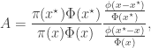
 using a bootstrap filter, and then accepting the proposal with probability
  , where
  is the
 is the bootstrap filter’s estimate of marginal likelihood for the new path, and
  is the estimate associated with the current path. Again using notation from the
 . Again, be sure to see the previous post for the explanation.
 rather than the exact conditional distribution
![\displaystyle \frac{\tilde{q}(\mathbf{x}_0,\ldots,\mathbf{x}_T,\mathbf{a}_0,\ldots,\mathbf{a}_{T-1})} {\displaystyle p(x_0^{b_0^k})\left[\prod_{t=0}^{T-1} \pi_t^{b_t^k}p\left(x_{t+1}^{b_{t+1}^k}|x_t^{b_t^k}\right)\right]}](https://s0.wp.com/latex.php?latex=%5Cdisplaystyle+%5Cfrac%7B%5Ctilde%7Bq%7D%28%5Cmathbf%7Bx%7D_0%2C%5Cldots%2C%5Cmathbf%7Bx%7D_T%2C%5Cmathbf%7Ba%7D_0%2C%5Cldots%2C%5Cmathbf%7Ba%7D_%7BT-1%7D%29%7D+%7B%5Cdisplaystyle+p%28x_0%5E%7Bb_0%5Ek%7D%29%5Cleft%5B%5Cprod_%7Bt%3D0%7D%5E%7BT-1%7D+%5Cpi_t%5E%7Bb_t%5Ek%7Dp%5Cleft%28x_%7Bt%2B1%7D%5E%7Bb_%7Bt%2B1%7D%5Ek%7D%7Cx_t%5E%7Bb_t%5Ek%7D%5Cright%29%5Cright%5D%7D&bg=ffffff&fg=333333&s=0&c=20201002) .
. paths, of which the conditioned-on trajectory is one.
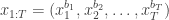 be the path that is to be conditioned on, with ancestral lineage
  . Then, for
  , sample
  and set
  . Now suppose that at time
  we have a weighted sample from
  . First resample by sampling
 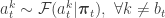 . Next sample
  . Then for all
  set
set 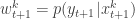 and normalise with
 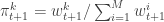 . Propagate this weighted set of particles to the next time point. At time
  select a single trajectory by sampling
  .
. of the
  random variables in the augmented state space at each iteration. Since the block of variables to be updated is random, this defines an ergodic sampler for
  particles, and we have explained why the marginal distribution of the selected trajectory is the exact conditional distribution.
 and the currently sampled path,
 . The potential function
  corresponds to the probability density function
 in R with the following code

 , the chain fails to jump to the second mode at all during this particular run of 100,000 iterations. That’s a problem if we are really interested in sampling from distributions like this. Of course, for this particular problem, there are all kinds of ways to fix this sampler, but the point is to try and develop methods that will work in high-dimensional situations where we cannot just “look” at what is going wrong.
 . In the context of Bayesian inference, tempering using the “power posterior” can often be more natural and useful (to be discussed in a subsequent post).
  and the other with target
  . We can consider these chains to be evolving together, with joint target
  . The updates chosen to update the within-chain states will obviously preserve this joint target. Now we consider how to swap states between the two chains without destroying the target. We simply propose a swap of
  to
to  , where
  and
and  . We are proposing this move as a standard Metropolis-Hastings update of the joint chain. We may therefore wonder about exactly what the proposal density for this move is. In fact, it is a point mass at the swapped values, and therefore has density


 target distribution, with density
 will be generated from
 is the standard normal density. This proposed new value is accepted with probability

 without checking the sign of
  distribution). So really we should check the sign of
  should be rejected. With the above code, such values are indeed rejected, and the sampler advances to the next iteration. However, in more complex samplers, where an update like this might be one tiny part of a massive sampler with a very high-dimensional state space, it seems like a bit of a "waste" of a MH move to just propose a negative value, throw it away, and move on. Evidently, it seems tempting, therefore, to keep on sampling

 is the standard normal CDF. Consequently, the correct acceptance ratio to use with this proposal is


 . On the other hand, the PMMH algorithm is an MCMC algorithm which targets the full joint posterior distribution
  ). Below I will describe the algorithm and explain why it works, but first it is necessary to understand the relationship between marginal, joint and “likelihood-free” MCMC updating schemes for such latent variable models.
 is proposed from
  and accepted with probability
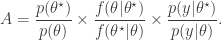
 required in the acceptance ratio is often difficult to compute.
 even when we can’t evaluate it, or marginalise
  . The pair
  is then jointly accepted with ratio
 . The pair
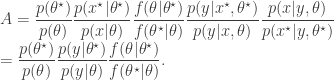
 , as the algorithms above. First, a proposed new
  is accepted using the Metropolis-Hastings ratio
 is the particle filter’s (unbiased) estimate of marginal likelihood, described in the previous post, and below. Note that this approach tends to the perfect joint/marginal updating scheme as the number of particles used in the filter tends to infinity. Note also that for a single particle, the particle filter just blindly forward simulates from
  and that the filter’s estimate of marginal likelihood is just the observed data likelihood
  leading precisely to the simple likelihood-free scheme. To understand for an arbitrary finite number of particles,
  ,
,  ,
,  . Initialise the particle filter with
  , where
  and
and  is undefined). Now suppose at time
  . First resample by sampling
  ,
,  . Here we use
  for the discrete distribution on
  with probability mass function
  . Next sample
  . Set
. Set  to the next step… We define the filter’s estimate of likelihood as
 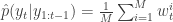 and
and 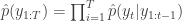 . See
. See ![\displaystyle \tilde{q}(\mathbf{x}_0,\ldots,\mathbf{x}_T,\mathbf{a}_0,\ldots,\mathbf{a}_{T-1}) = \left[\prod_{k=1}^M p(x_0^k)\right] \left[\prod_{t=0}^{T-1} \prod_{k=1}^M \pi_t^{a_t^k} p(x_{t+1}^k|x_t^{a_t^k}) \right]](https://s0.wp.com/latex.php?latex=%5Cdisplaystyle++%5Ctilde%7Bq%7D%28%5Cmathbf%7Bx%7D_0%2C%5Cldots%2C%5Cmathbf%7Bx%7D_T%2C%5Cmathbf%7Ba%7D_0%2C%5Cldots%2C%5Cmathbf%7Ba%7D_%7BT-1%7D%29++%3D+%5Cleft%5B%5Cprod_%7Bk%3D1%7D%5EM+p%28x_0%5Ek%29%5Cright%5D+%5Cleft%5B%5Cprod_%7Bt%3D0%7D%5E%7BT-1%7D++++%5Cprod_%7Bk%3D1%7D%5EM+%5Cpi_t%5E%7Ba_t%5Ek%7D+p%28x_%7Bt%2B1%7D%5Ek%7Cx_t%5E%7Ba_t%5Ek%7D%29+%5Cright%5D++&bg=ffffff&fg=333333&s=0&c=20201002)
 from
from  giving the joint density

 , and
, and  . If we now think about the structure of the PMMH algorithm, our proposal on the space of all random variables in the problem is in fact

 when we consider just the parameters and the selected trajectory. But if we consider the terms in the joint distribution of the proposal corresponding to the trajectory selected by
 ![\displaystyle p_\theta(x_0^{b_0^{k'}})\left[\prod_{t=0}^{T-1} \pi_t^{b_t^{k'}} p_\theta(x_{t+1}^{b_{t+1}^{k'}}|x_t^{b_t^{k'}})\right]\pi_T^{k'} = p_\theta(x_{0:T}^{k'})\prod_{t=0}^T \pi_t^{b_t^{k'}}](https://s0.wp.com/latex.php?latex=%5Cdisplaystyle++p_%5Ctheta%28x_0%5E%7Bb_0%5E%7Bk%27%7D%7D%29%5Cleft%5B%5Cprod_%7Bt%3D0%7D%5E%7BT-1%7D+%5Cpi_t%5E%7Bb_t%5E%7Bk%27%7D%7D++++p_%5Ctheta%28x_%7Bt%2B1%7D%5E%7Bb_%7Bt%2B1%7D%5E%7Bk%27%7D%7D%7Cx_t%5E%7Bb_t%5E%7Bk%27%7D%7D%29%5Cright%5D%5Cpi_T%5E%7Bk%27%7D++%3D++p_%5Ctheta%28x_%7B0%3AT%7D%5E%7Bk%27%7D%29%5Cprod_%7Bt%3D0%7D%5ET+%5Cpi_t%5E%7Bb_t%5E%7Bk%27%7D%7D++&bg=ffffff&fg=333333&s=0&c=20201002)
 in terms of the unnormalised weights, simplifies to
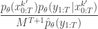
 in the acceptance ratio, we knock out the normalising constant, allowing all of the other terms in the proposal to be marginalised away. In other words, the target of the chain can be written as proportional to

 using a proposal
  . As explained previously, the required Metropolis-Hastings acceptance ratio will take the form
 , can be computed. We can obviously just substitute this estimate into the acceptance ratio to get
 , where the expectation is with respect to the Monte-Carlo error for a given fixed value of
  , representing the noise in the Monte-Carlo estimate of
  (note that in an abuse of notation, the function
  is unrelated to
  , where
  is a constant independent of
  , we have the (typical) special case of
  , but we will consider relaxing this constraint later.
  is being proposed in addition to a new value for
  , it is clear that the proposal generates
  from the density
 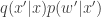 , and we can re-write our “approximate” acceptance ratio as
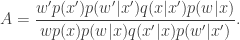

 , but the marginal for

