Introduction
In the previous post I explained how one can use an unbiased estimate of marginal likelihood derived from a particle filter within a Metropolis-Hastings MCMC algorithm in order to construct an exact pseudo-marginal MCMC scheme for the posterior distribution of the model parameters given some time course data. This idea is closely related to that of the particle marginal Metropolis-Hastings (PMMH) algorithm of Andreiu et al (2010), but not really exactly the same. This is because for a Bayesian model with parameters  , latent variables
  and data
  , of the form

the pseudo-marginal algorithm which exploits the fact that the particle filter’s estimate of likelihood is unbiased is an MCMC algorithm which directly targets the marginal posterior distribution  . On the other hand, the PMMH algorithm is an MCMC algorithm which targets the full joint posterior distribution
  . Now, the PMMH scheme does reduce to the pseudo-marginal scheme if samples of are not generated and stored in the state of the Markov chain, and it certainly is the case that the pseudo-marginal algorithm gives some insight into why the PMMH algorithm works. However, the PMMH algorithm is much more powerful, as it solves the “smoothing” and parameter estimation problem simultaneously and exactly, including the “initial value” problem (computing the posterior distribution of the initial state,
  ). Below I will describe the algorithm and explain why it works, but first it is necessary to understand the relationship between marginal, joint and “likelihood-free” MCMC updating schemes for such latent variable models.
MCMC for latent variable models
Marginal approach
If we want to target directly, we can use a Metropolis-Hastings scheme with a fairly arbitrary proposal distribution for exploring , where a new  is proposed from
  and accepted with probability
  , where
As previously discussed, the problem with this scheme is that the marginal likelihood  required in the acceptance ratio is often difficult to compute.
Likelihood-free MCMC
A simple “likelihood-free” scheme targets the full joint posterior distribution . It works by exploiting the fact that we can often simulate from the model for the latent variables  even when we can’t evaluate it, or marginalise out of the problem. Here the Metropolis-Hastings proposal is constructed in two stages. First, a proposed new is sampled from and then a corresponding
  is simulated from the model
  . The pair
  is then jointly accepted with ratio

The proposal mechanism ensures that the proposed is consistent with the proposed , and so the procedure can work provided that the dimension of the data is low. However, in order to work well more generally, we would want the proposed latent variables to be consistent with the data as well as the model parameters.
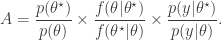
Ideal joint update
Motivated by the likelihood-free scheme, we would really like to target the joint posterior by first proposing from and then a corresponding from the conditional distribution  . The pair is then jointly accepted with ratio
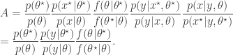
Notice how the acceptance ratio simplifies, using the basic marginal likelihood identity (BMI) of Chib (1995), and drops out of the ratio completely in order to give exactly the ratio used for the marginal updating scheme. Thus, the “ideal” joint updating scheme reduces to the marginal updating scheme if is not sampled and stored as a component of the Markov chain.
Understanding the relationship between these schemes is useful for understanding the PMMH algorithm. Indeed, we will see that the “ideal” joint updating scheme (and the marginal scheme) corresponds to PMMH using infinitely many particles in the particle filter, and that the likelihood-free scheme corresponds to PMMH using exactly one particle in the particle filter. For an intermediate number of particles, the PMMH scheme is a compromise between the “ideal” scheme and the “blind” likelihood-free scheme, but is always likelihood-free (when used with a bootstrap particle filter) and always has an acceptance ratio leaving the exact posterior invariant.
The PMMH algorithm
The algorithm
The PMMH algorithm is an MCMC algorithm for state space models jointly updating and  , as the algorithms above. First, a proposed new is generated from a proposal , and then a corresponding
  is generated by running a bootstrap particle filter (as described in the previous post, and below) using the proposed new model parameters, , and selecting a single trajectory by sampling once from the final set of particles using the final set of weights. This proposed pair
  is accepted using the Metropolis-Hastings ratio

where  is the particle filter’s (unbiased) estimate of marginal likelihood, described in the previous post, and below. Note that this approach tends to the perfect joint/marginal updating scheme as the number of particles used in the filter tends to infinity. Note also that for a single particle, the particle filter just blindly forward simulates from
  and that the filter’s estimate of marginal likelihood is just the observed data likelihood
  leading precisely to the simple likelihood-free scheme. To understand for an arbitrary finite number of particles,
  , one needs to think carefully about the structure of the particle filter.
Why it works
To understand why PMMH works, it is necessary to think about the joint distribution of all random variables used in the bootstrap particle filter. To this end, it is helpful to re-visit the particle filter, thinking carefully about the resampling and propagation steps.
First introduce notation for the “particle cloud”:  ,
,  ,
,  . Initialise the particle filter with
  , where
  and
and  (note that
  is undefined). Now suppose at time
  we have a sample from
  :
:  . First resample by sampling
  ,
,  . Here we use
  for the discrete distribution on
  with probability mass function
  . Next sample
  . Set
. Set 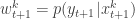 and
and 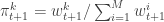 . Finally, propagate
  to the next step… We define the filter’s estimate of likelihood as
 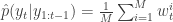 and
and 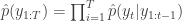 . See Doucet et al (2001) for further theoretical background on particle filters and SMC more generally.
Describing the filter carefully as above allows us to write down the joint density of all random variables in the filter as
![\displaystyle \tilde{q}(\mathbf{x}_0,\ldots,\mathbf{x}_T,\mathbf{a}_0,\ldots,\mathbf{a}_{T-1}) = \left[\prod_{k=1}^M p(x_0^k)\right] \left[\prod_{t=0}^{T-1} \prod_{k=1}^M \pi_t^{a_t^k} p(x_{t+1}^k|x_t^{a_t^k}) \right]](https://s0.wp.com/latex.php?latex=%5Cdisplaystyle++%5Ctilde%7Bq%7D%28%5Cmathbf%7Bx%7D_0%2C%5Cldots%2C%5Cmathbf%7Bx%7D_T%2C%5Cmathbf%7Ba%7D_0%2C%5Cldots%2C%5Cmathbf%7Ba%7D_%7BT-1%7D%29++%3D+%5Cleft%5B%5Cprod_%7Bk%3D1%7D%5EM+p%28x_0%5Ek%29%5Cright%5D+%5Cleft%5B%5Cprod_%7Bt%3D0%7D%5E%7BT-1%7D++++%5Cprod_%7Bk%3D1%7D%5EM+%5Cpi_t%5E%7Ba_t%5Ek%7D+p%28x_%7Bt%2B1%7D%5Ek%7Cx_t%5E%7Ba_t%5Ek%7D%29+%5Cright%5D++&bg=ffffff&fg=333333&s=0&c=20201002)
For PMMH we also sample a final index  from
from  giving the joint density

We write the final selected trajectory as

where  , and
, and  . If we now think about the structure of the PMMH algorithm, our proposal on the space of all random variables in the problem is in fact

and by considering the proposal and the acceptance ratio, it is clear that detailed balance for the chain is satisfied by the target with density proportional to

We want to show that this target marginalises down to the correct posterior  when we consider just the parameters and the selected trajectory. But if we consider the terms in the joint distribution of the proposal corresponding to the trajectory selected by , this is given by
![\displaystyle p_\theta(x_0^{b_0^{k'}})\left[\prod_{t=0}^{T-1} \pi_t^{b_t^{k'}} p_\theta(x_{t+1}^{b_{t+1}^{k'}}|x_t^{b_t^{k'}})\right]\pi_T^{k'} = p_\theta(x_{0:T}^{k'})\prod_{t=0}^T \pi_t^{b_t^{k'}}](https://s0.wp.com/latex.php?latex=%5Cdisplaystyle++p_%5Ctheta%28x_0%5E%7Bb_0%5E%7Bk%27%7D%7D%29%5Cleft%5B%5Cprod_%7Bt%3D0%7D%5E%7BT-1%7D+%5Cpi_t%5E%7Bb_t%5E%7Bk%27%7D%7D++++p_%5Ctheta%28x_%7Bt%2B1%7D%5E%7Bb_%7Bt%2B1%7D%5E%7Bk%27%7D%7D%7Cx_t%5E%7Bb_t%5E%7Bk%27%7D%7D%29%5Cright%5D%5Cpi_T%5E%7Bk%27%7D++%3D++p_%5Ctheta%28x_%7B0%3AT%7D%5E%7Bk%27%7D%29%5Cprod_%7Bt%3D0%7D%5ET+%5Cpi_t%5E%7Bb_t%5E%7Bk%27%7D%7D++&bg=ffffff&fg=333333&s=0&c=20201002)
which, by expanding the  in terms of the unnormalised weights, simplifies to
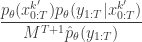
It is worth dwelling on this result, as this is the key insight required to understand why the PMMH algorithm works. The whole point is that the terms in the joint density of the proposal corresponding to the selected trajectory exactly represent the required joint distribution modulo a couple of normalising constants, one of which is the particle filter’s estimate of marginal likelihood. Thus, by including  in the acceptance ratio, we knock out the normalising constant, allowing all of the other terms in the proposal to be marginalised away. In other words, the target of the chain can be written as proportional to

The other terms are all probabilities of random variables which do not occur elsewhere in the target, and hence can all be marginalised away to leave the correct posterior

Thus the PMMH algorithm targets the correct posterior for any number of particles, . Also note the implied uniform distribution on the selected indices in the target.
I will give some code examples in a future post.

This is a really great and clear explanation of pMCMC. Even though I’ve read the Andrieu et al. paper a couple of times, this really helped clear up a few things for me. I’ve actually been trying to use pMCMC to fit nonlinear epidemiological models to time series data. I implemented a basic version of the algorithm in Matlab and it seemed to work well even though my epi models have what I consider to be a large state space. But it was slow… painfully slow actually even with ~100 particles. Since you seem to be a fan of using Java for numerical computation, I was wondering if you’ve implemented the pMCMC algorithm in Java, and if so, if you have code you could share? I’m just starting to make the switch to Java so it would be great if I could see how somebody else would code this.
Thanks!!
David Rasmussen
Biology Dept.
Duke University
Durham, NC, USA
Thanks for your feedback. Regarding a Java implementation – not yet! If you’d like to see how to do this in R (which will not be any faster than Matlab), I am currently finishing off an R package “smfsb” for the second edition of my book which includes a pMCMC example. The installation instructions are here: http://www.staff.ncl.ac.uk/d.j.wilkinson/smfsb/2e/ and running ‘demo(“PMCMC”)’ will give a demo of how to do it. It may be of interest to see how I structured the code to make it easy to bolt together different models, simulation algorithms, particle filters and MCMC schemes (using function closures). I’ll talk about that in future posts. The way it is structured, it should port easily to any reasonable functional or O-O language (including Scala and Java). Porting the framework to Java is on my (very long) list of things to do, but don’t hold your breath! Regards,
Thanks! I’m looking forward to your upcoming posts, and book.
A bit off-topic question: your book (of 2011 year edition) should arrive to me in a few weeks, and I wonder what additional reading may be advised to a software engineer gradually shifting towards systems biology? Which books (or other resources) do you consider as a must, which ones to read after?
This is actually a tricky question, as systems biology is very broad, so the answer really depends on the kind of systems biology that you are shifting towards. You could do worse than to start with Voit’s book: http://amzn.to/1dQ88X2 – which is quite nicely done, as a starting point. But going beyond that is likely to be very topic specific.
Thank you for advice! It seems to be something I was looking for, field is indeed too broad.
This may be a dumb question, but in deriving the last line of your calculations, what happened to the p(y_{1:T}) in the denominator of the final posterior?
err, numerator, not denominator.
If you are referring to the genuine p(y_{1:T}), then this is just the usual constant of proportionality which will cancel out of the MH ratio. Note that this is different to p(y_{1:T}|theta), which I’ve written as p_theta(y_{1:T}), which you do have to carefully keep track of.
Assuming that theta is known, is it correct to say that the samples of x1T are what you would get if you ran MH using the filtering distribution as a proposal density.
If so, if the filtering and smoothing distribution have a high KL-divergence (because the hidden state transition is slowly mixing for instance) would it be fair to say that samples of x1T will get trapped in local maxima for many iterations, making the acceptance rate very small?
Are there techniques that alleviate this problem by using a proposal distribution that depends on the current x1T, but which are capable of getting reasonable acceptance rates?
No, the proposals are from the smoothing distribution. Nevertheless, you might be interested in particle Gibbs, and techniques to address particle degeneracy in particle Gibbs, such as ancestral sampling. My introduction to particle Gibbs is a reasonable place to start: https://darrenjw.wordpress.com/2014/01/25/introduction-to-the-particle-gibbs-sampler/
Oh, but that most be true only for an infinite number of particles then… Is it then that the proposal is from some intermediate distribution between filtering and smoothing when there are a finite number of particles?
OK, to be more precise, the proposal is from the usual particle approximation to the smoothing distribution, which tends to the true smoothing distribution as the number of particles increases. But it is not the filtering distribution.
OK, it’s not even the filtering distribution if n=1 either, is it? Only for the marginal P(x0)…
Actually, for n=1 particle, you just have a blind “likelihood free” forward simulation from the model (ignoring the data). But in that case I guess it is the 1-particle approximation to both the filtering and smoothing distributions (but neither are any good!).
Oh right of course. I do have an intuition that the greater the divergence between filtering and smoothing, the higher the autocorrelation in samples from x1T, but I can’t quite put my finger on why.