Introduction
In the previous post I explained how one can use an unbiased estimate of marginal likelihood derived from a particle filter within a Metropolis-Hastings MCMC algorithm in order to construct an exact pseudo-marginal MCMC scheme for the posterior distribution of the model parameters given some time course data. This idea is closely related to that of the particle marginal Metropolis-Hastings (PMMH) algorithm of Andreiu et al (2010), but not really exactly the same. This is because for a Bayesian model with parameters  , latent variables
  and data
  , of the form

the pseudo-marginal algorithm which exploits the fact that the particle filter’s estimate of likelihood is unbiased is an MCMC algorithm which directly targets the marginal posterior distribution  . On the other hand, the PMMH algorithm is an MCMC algorithm which targets the full joint posterior distribution
  . Now, the PMMH scheme does reduce to the pseudo-marginal scheme if samples of are not generated and stored in the state of the Markov chain, and it certainly is the case that the pseudo-marginal algorithm gives some insight into why the PMMH algorithm works. However, the PMMH algorithm is much more powerful, as it solves the “smoothing” and parameter estimation problem simultaneously and exactly, including the “initial value” problem (computing the posterior distribution of the initial state,
  ). Below I will describe the algorithm and explain why it works, but first it is necessary to understand the relationship between marginal, joint and “likelihood-free” MCMC updating schemes for such latent variable models.
MCMC for latent variable models
Marginal approach
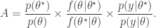
If we want to target directly, we can use a Metropolis-Hastings scheme with a fairly arbitrary proposal distribution for exploring , where a new  is proposed from
  and accepted with probability
  , where
As previously discussed, the problem with this scheme is that the marginal likelihood  required in the acceptance ratio is often difficult to compute.
Likelihood-free MCMC
A simple “likelihood-free” scheme targets the full joint posterior distribution . It works by exploiting the fact that we can often simulate from the model for the latent variables  even when we can’t evaluate it, or marginalise out of the problem. Here the Metropolis-Hastings proposal is constructed in two stages. First, a proposed new is sampled from and then a corresponding
  is simulated from the model
  . The pair
  is then jointly accepted with ratio

The proposal mechanism ensures that the proposed is consistent with the proposed , and so the procedure can work provided that the dimension of the data is low. However, in order to work well more generally, we would want the proposed latent variables to be consistent with the data as well as the model parameters.
Ideal joint update
Motivated by the likelihood-free scheme, we would really like to target the joint posterior by first proposing from and then a corresponding from the conditional distribution  . The pair is then jointly accepted with ratio
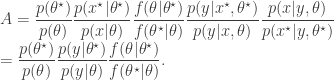
Notice how the acceptance ratio simplifies, using the basic marginal likelihood identity (BMI) of Chib (1995), and drops out of the ratio completely in order to give exactly the ratio used for the marginal updating scheme. Thus, the “ideal” joint updating scheme reduces to the marginal updating scheme if is not sampled and stored as a component of the Markov chain.
Understanding the relationship between these schemes is useful for understanding the PMMH algorithm. Indeed, we will see that the “ideal” joint updating scheme (and the marginal scheme) corresponds to PMMH using infinitely many particles in the particle filter, and that the likelihood-free scheme corresponds to PMMH using exactly one particle in the particle filter. For an intermediate number of particles, the PMMH scheme is a compromise between the “ideal” scheme and the “blind” likelihood-free scheme, but is always likelihood-free (when used with a bootstrap particle filter) and always has an acceptance ratio leaving the exact posterior invariant.
The PMMH algorithm
The algorithm
The PMMH algorithm is an MCMC algorithm for state space models jointly updating and  , as the algorithms above. First, a proposed new is generated from a proposal , and then a corresponding
  is generated by running a bootstrap particle filter (as described in the previous post, and below) using the proposed new model parameters, , and selecting a single trajectory by sampling once from the final set of particles using the final set of weights. This proposed pair
  is accepted using the Metropolis-Hastings ratio

where  is the particle filter’s (unbiased) estimate of marginal likelihood, described in the previous post, and below. Note that this approach tends to the perfect joint/marginal updating scheme as the number of particles used in the filter tends to infinity. Note also that for a single particle, the particle filter just blindly forward simulates from
  and that the filter’s estimate of marginal likelihood is just the observed data likelihood
  leading precisely to the simple likelihood-free scheme. To understand for an arbitrary finite number of particles,
  , one needs to think carefully about the structure of the particle filter.
Why it works
To understand why PMMH works, it is necessary to think about the joint distribution of all random variables used in the bootstrap particle filter. To this end, it is helpful to re-visit the particle filter, thinking carefully about the resampling and propagation steps.
First introduce notation for the “particle cloud”:  ,
,  ,
,  . Initialise the particle filter with
  , where
  and
and  (note that
  is undefined). Now suppose at time
  we have a sample from
  :
:  . First resample by sampling
  ,
,  . Here we use
  for the discrete distribution on
  with probability mass function
  . Next sample
  . Set
. Set 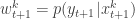 and
and 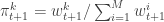 . Finally, propagate
  to the next step… We define the filter’s estimate of likelihood as
  and
and  . See Doucet et al (2001) for further theoretical background on particle filters and SMC more generally.
Describing the filter carefully as above allows us to write down the joint density of all random variables in the filter as
![\displaystyle \tilde{q}(\mathbf{x}_0,\ldots,\mathbf{x}_T,\mathbf{a}_0,\ldots,\mathbf{a}_{T-1}) = \left[\prod_{k=1}^M p(x_0^k)\right] \left[\prod_{t=0}^{T-1} \prod_{k=1}^M \pi_t^{a_t^k} p(x_{t+1}^k|x_t^{a_t^k}) \right]](https://s0.wp.com/latex.php?latex=%5Cdisplaystyle++%5Ctilde%7Bq%7D%28%5Cmathbf%7Bx%7D_0%2C%5Cldots%2C%5Cmathbf%7Bx%7D_T%2C%5Cmathbf%7Ba%7D_0%2C%5Cldots%2C%5Cmathbf%7Ba%7D_%7BT-1%7D%29++%3D+%5Cleft%5B%5Cprod_%7Bk%3D1%7D%5EM+p%28x_0%5Ek%29%5Cright%5D+%5Cleft%5B%5Cprod_%7Bt%3D0%7D%5E%7BT-1%7D++++%5Cprod_%7Bk%3D1%7D%5EM+%5Cpi_t%5E%7Ba_t%5Ek%7D+p%28x_%7Bt%2B1%7D%5Ek%7Cx_t%5E%7Ba_t%5Ek%7D%29+%5Cright%5D++&bg=ffffff&fg=333333&s=0&c=20201002)
For PMMH we also sample a final index  from
from  giving the joint density

We write the final selected trajectory as

where  , and
, and  . If we now think about the structure of the PMMH algorithm, our proposal on the space of all random variables in the problem is in fact

and by considering the proposal and the acceptance ratio, it is clear that detailed balance for the chain is satisfied by the target with density proportional to

We want to show that this target marginalises down to the correct posterior  when we consider just the parameters and the selected trajectory. But if we consider the terms in the joint distribution of the proposal corresponding to the trajectory selected by , this is given by
![\displaystyle p_\theta(x_0^{b_0^{k'}})\left[\prod_{t=0}^{T-1} \pi_t^{b_t^{k'}} p_\theta(x_{t+1}^{b_{t+1}^{k'}}|x_t^{b_t^{k'}})\right]\pi_T^{k'} = p_\theta(x_{0:T}^{k'})\prod_{t=0}^T \pi_t^{b_t^{k'}}](https://s0.wp.com/latex.php?latex=%5Cdisplaystyle++p_%5Ctheta%28x_0%5E%7Bb_0%5E%7Bk%27%7D%7D%29%5Cleft%5B%5Cprod_%7Bt%3D0%7D%5E%7BT-1%7D+%5Cpi_t%5E%7Bb_t%5E%7Bk%27%7D%7D++++p_%5Ctheta%28x_%7Bt%2B1%7D%5E%7Bb_%7Bt%2B1%7D%5E%7Bk%27%7D%7D%7Cx_t%5E%7Bb_t%5E%7Bk%27%7D%7D%29%5Cright%5D%5Cpi_T%5E%7Bk%27%7D++%3D++p_%5Ctheta%28x_%7B0%3AT%7D%5E%7Bk%27%7D%29%5Cprod_%7Bt%3D0%7D%5ET+%5Cpi_t%5E%7Bb_t%5E%7Bk%27%7D%7D++&bg=ffffff&fg=333333&s=0&c=20201002)
which, by expanding the  in terms of the unnormalised weights, simplifies to
It is worth dwelling on this result, as this is the key insight required to understand why the PMMH algorithm works. The whole point is that the terms in the joint density of the proposal corresponding to the selected trajectory exactly represent the required joint distribution modulo a couple of normalising constants, one of which is the particle filter’s estimate of marginal likelihood. Thus, by including  in the acceptance ratio, we knock out the normalising constant, allowing all of the other terms in the proposal to be marginalised away. In other words, the target of the chain can be written as proportional to

The other terms are all probabilities of random variables which do not occur elsewhere in the target, and hence can all be marginalised away to leave the correct posterior

Thus the PMMH algorithm targets the correct posterior for any number of particles, . Also note the implied uniform distribution on the selected indices in the target.
I will give some code examples in a future post.
