The pseudo-marginal approach to MCMC for Bayesian inference
In a previous post I described a generalisation of the Metropolis Hastings MCMC algorithm which uses unbiased Monte Carlo estimates of likelihood in the acceptance ratio, but is nevertheless exact, when considered as a pseudo-marginal approach to “exact approximate” MCMC. To be useful in the context of Bayesian inference, we need to be able to compute unbiased estimates of the (marginal) likelihood of the data given some proposed model parameters with any “latent variables” integrated out.
To be more precise, consider a model for data with parameters of the form together with a prior on , , giving a joint model
Suppose now that interest is in the posterior distribution
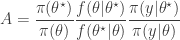
We can construct a fairly generic (marginal) MCMC scheme for this posterior by first proposing from some fairly arbitrary proposal distribution and then accepting the value with probability where
This method is great provided that the (marginal) likelihood of the data is available to us analytically, but in many (most) interesting models it is not. However, in the previous post I explained why substituting in a Monte Carlo estimate will still lead to the exact posterior if the estimate is unbiased in the sense that . Consequently, sources of (cheap) unbiased Monte Carlo estimates of (marginal) likelihood are of potential interest in the development of exact MCMC algorithms.
Latent variables and marginalisation
Often the reason that we cannot evaluate is that there are latent variables in the problem, and the model for the data is conditional on those latent variables. Explicitly, if we denote the latent variables by , then the joint distribution for the model takes the form
Now since
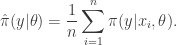
there is a simple and obvious Monte Carlo strategy for estimating provided that we can evaluate and simulate realisations from . That is, simulate values from for some suitably large , and then put
It is clear by the law of large numbers that this estimate will converge to as . That is, is a consistent estimate of . However, a moment’s thought reveals that this estimate is not only consistent, but also unbiased, since each term in the sum has expectation . This simple Monte Carlo estimate of likelihood can therefore be substituted into a Metropolis-Hastings acceptance ratio without affecting the (marginal) target distribution of the Markov chain. Note that this estimate of marginal likelihood is sometimes referred to as the Rao-Blackwellised estimate, due to its connection with the Rao-Blackwell theorem.
Importance sampling
Suppose now that we cannot sample values directly from , but can sample instead from a distribution having the same support as . We can then instead produce an importance sampling estimate for by noting that
Consequently, samples from can be used to construct the estimate
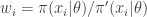
which again is clearly both consistent and unbiased. This estimate is often written
where . The weights, , are known as importance weights.
Importance resampling
An idea closely related to that of importance sampling is that of importance resampling where importance weights are used to resample a sample in order to equalise the weights, often prior to a further round of weighting and resampling. The basic idea is to generate an approximate sample from a target density using values sampled from an auxiliary distribution , where we now supress any dependence of the distributions on model parameters, .
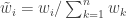
First generate a sample from and compute weights . Then compute normalised weights . Generate a new sample of size by sampling times with replacement from the original sample with the probability of choosing each value determined by its normalised weight.
As an example, consider using a sample from the Cauchy distribution as an auxiliary distribution for approximately sampling standard normal random quantities. We can do this using a few lines of R as follows.
Note that we don’t actually need to compute the normalised weights, as the sample function will do this for us. Note also that the average weight will be close to one. It should be clear that the expected value of the weights will be exactly 1 when both the target and auxiliary densities are correctly normalised. Also note that the procedure can be used when one or both of the densities are not correctly normalised, since the weights will be normalised prior to sampling anyway. Note that in this case the expected weight will be the (ratio of) normalising constant(s), and so looking at the average weight will give an estimate of the normalising constant.
Note that the importance sampling procedure is approximate. Unlike a technique such as rejection sampling, which leads to samples having exactly the correct distribution, this is not the case here. Indeed, it is clear that in the case, the final sample will be exactly drawn from the auxiliary and not the target. The procedure is asymptotic, in that it improves as the sample size increases, tending to the exact target as .
We can understand why importance resampling works by first considering the univariate case, using correctly normalised densities. Consider a very large number of particles, . The proportion of the auxiliary samples falling in a small interval will be , corresponding to roughly particles. The weight for each of those particles will be , and since the expected weight of a random particle is 1, the sum of all weights will be (roughly) , leading to normalised weights for the particles near of . The combined weight of all particles in is therefore . Clearly then, when we resample times we expect to select roughly particles from this interval. This corresponds to a proportion , corresponding to a density of in the final sample.
Obviously the above argument is very informal, but can be tightened up into a reasonably rigorous proof for the 1d case without too much effort, and the multivariate extension is also reasonably clear.
The bootstrap particle filter
The bootstrap particle filter is an iterative method for carrying out Bayesian inference for dynamic state space (partially observed Markov process) models, sometimes also known as hidden Markov models (HMMs). Here, an unobserved Markov process, governed by a transition kernel is partially observed via some measurement model leading to data . The idea is to make inference for the hidden states given the data . The method is a very simple application of the importance resampling technique. At each time, , we assume that we have a (approximate) sample from and use importance resampling to generate an approximate sample from .
More precisely, the procedure is initialised with a sample from with uniform normalised weights . Then suppose that we have a weighted sample from . First generate an equally weighted sample by resampling with replacement times to obtain (giving an approximate random sample from ). Note that each sample is independently drawn from . Next propagate each particle forward according to the Markov process model by sampling (giving an approximate random sample from ). Then for each of the new particles, compute a weight , and then a normalised weight .
It is clear from our understanding of importance resampling that these weights are appropriate for representing a sample from , and so the particles and weights can be propagated forward to the next time point. It is also clear that the average weight at each time gives an estimate of the marginal likelihood of the current data point given the data so far. So we define
and
Again, from our understanding of importance resampling, it should be reasonably clear that is a consistent estimator of . It is much less clear, but nevertheless true that this estimator is also unbiased. The standard reference for this fact is Del Moral (2004), but this is a rather technical monograph. A much more accessible proof (for a very general particle filter) is given in Pitt et al (2011).
It should therefore be clear that if one is interested in developing MCMC algorithms for state space models, one can use a pseudo-marginal MCMC scheme, substituting in from a bootstrap particle filter in place of . This turns out to be a simple special case of the particle marginal Metropolis-Hastings (PMMH) algorithm described in Andreiu et al (2010). However, the PMMH algorithm in fact has the full joint posterior as its target. I will explain the PMMH algorithm in a subsequent post.
In this post I will try and explain an important idea behind some recent developments in MCMC theory. First, let me give some motivation. Suppose you are trying to implement a Metropolis-Hastings algorithm, as discussed in a previous post (required reading!), but a key likelihood term needed for the acceptance ratio is difficult to evaluate (most likely it is a marginal likelihood of some sort). If it is possible to obtain a Monte-Carlo estimate for that likelihood term (which it sometimes is, for example, using importance sampling), one could obviously just plug it in to the acceptance ratio and hope for the best. What is not at all obvious is that if your Monte-Carlo estimate satisfies some fairly weak property then the equilibrium distribution of the Markov chain will remain exactly as it would be if the exact likelihood had been available. Furthermore, it is exact even if the Monte-Carlo estimate is very noisy and imprecise (though the mixing of the chain will be poorer in this case). This is the “exact approximate” pseudo-marginal MCMC approach. To give credit where it is due, the idea was first introduced by Mark Beaumont in Beaumont (2003), where he was using an importance sampling based approximate likelihood in the context of a statistical genetics example. This was later picked up by Christophe Andrieu and Gareth Roberts, who studied the technical properties of the approach in Andrieu and Roberts (2009). The idea is turning out to be useful in several contexts, and in particular, underpins the interesting new Particle MCMC algorithms of Andrieu et al (2010), which I will discuss in a future post. I’ve heard Mark, Christophe, Gareth and probably others present this concept, but this post is most strongly inspired by a talk that Christophe gave at the IMS 2010 meeting in Gothenburg this summer.
The pseudo-marginal Metropolis-Hastings algorithm
Let’s focus on the simplest version of the problem, where we want to sample from a target using a proposal . As explained previously, the required Metropolis-Hastings acceptance ratio will take the form
Here we are assuming that is difficult to evaluate (usually because it is a marginalised version of some higher-dimensional distribution), but that a Monte-Carlo estimate of , which we shall denote , can be computed. We can obviously just substitute this estimate into the acceptance ratio to get
but it is not immediately clear that in many cases this will lead to the Markov chain having an equilibrium distribution that is exactly. It turns out that it is sufficient that the likelihood estimate, is non-negative, and unbiased, in the sense that , where the expectation is with respect to the Monte-Carlo error for a given fixed value of . In fact, as we shall see, this condition is actually a bit stronger than is really required.
Put , representing the noise in the Monte-Carlo estimate of , and suppose that (note that in an abuse of notation, the function is unrelated to ). The main condition we will assume is that , where is a constant independent of . In the case of , we have the (typical) special case of . For now, we will also assume that , but we will consider relaxing this constraint later.
The key to understanding the pseudo-marginal approach is to realise that at each iteration of the MCMC algorithm a new value of is being proposed in addition to a new value for . If we regard the proposal mechanism as a joint update of and , it is clear that the proposal generates from the density , and we can re-write our “approximate” acceptance ratio as
Inspection of this acceptance ratio reveals that the target of the chain must be (proportional to)
This is a joint density for , but the marginal for can be obtained by integrating over the range of with respect to . Using the fact that , this then clearly gives a density proportional to , and this is precisely the target that we require. Note that for this to work, we must keep the old value of from one iteration to the next – that is, we must keep and re-use our noisy value to include in the acceptance ratio for our next MCMC iteration – we should not compute a new Monte-Carlo estimate for the likelihood of the old state of the chain.
Examples
We will consider again the example from the previous post – simulation of a chain with a N(0,1) target using uniform innovations. Using R, the main MCMC loop takes the form
pmmcmc<-function(n=1000,alpha=0.5)
{
        vec=vector("numeric", n)
        x=0
        oldlik=noisydnorm(x)
        vec[1]=x
        for (i in 2:n) {
                innov=runif(1,-alpha,alpha)
                can=x+innov
                lik=noisydnorm(can)
                aprob=lik/oldlik
                u=runif(1)
                if (u < aprob) {
                        x=can
                        oldlik=lik
			}
                vec[i]=x
        }
        vec
}
Here we are assuming that we are unable to compute dnorm exactly, but instead only a Monte-Carlo estimate called noisydnorm. We can start with the following implementation
noisydnorm<-function(z)
{
	dnorm(z)*rexp(1,1)
}
Each time this function is called, it will return a non-negative random quantity whose expectation is dnorm(z). We can now run this code as follows.
So we see that we have exactly the right N(0,1) target, despite using the (very) noisy noisydnorm function in place of the dnorm function. This noisy likelihood function is clearly unbiased. However, as already discussed, a constant bias in the noise is also acceptable, as the following function shows.
noisydnorm<-function(z)
{
	dnorm(z)*rexp(1,2)
}
Re-running the code with this function also leads to the correct equilibrium distribution for the chain. However, it really does matter that the bias is independent of the state of the chain, as the following function shows.
Running with this function leads to the wrong equilibrium. However, it is OK for the distribution of the noise to depend on the state, as long as its expectation does not. The following function illustrates this.
This works just fine. So far we have been assuming that our noisy likelihood estimates are non-negative. This is clearly desirable, as otherwise we could wind up with negative Metropolis-Hasting ratios. However, as long as we are careful about exactly what we mean, even this non-negativity condition may be relaxed. The following function illustrates the point.
noisydnorm<-function(z)
{
	dnorm(z)*rnorm(1,1)
}
Despite the fact that this function will often produce negative values, the equilibrium distribution of the chain still seems to be correct! An even more spectacular example follows.
noisydnorm<-function(z)
{
	dnorm(z)*rnorm(1,0)
}
Astonishingly, this one works too, despite having an expected value of zero! However, the following doesn’t work, even though it too has a constant expectation of zero.
I don’t have time to explain exactly what is going on here, so the precise details are left as an exercise for the reader. Suffice to say that the key requirement is that it is the distribution of W conditioned to be non-negative which must have the constant bias property – something clearly violated by the final noisydnorm example.
Before finishing this post, it is worth re-emphasising the issue of re-using old Monte-Carlo estimates. The following function will not work (exactly), though in the case of good Monte-Carlo estimates will often work tolerably well.
approxmcmc<-function(n=1000,alpha=0.5)
{
        vec=vector("numeric", n)
        x=0
        vec[1]=x
        for (i in 2:n) {
                innov=runif(1,-alpha,alpha)
                can=x+innov
                lik=noisydnorm(can)
                oldlik=noisydnorm(x)
                aprob=lik/oldlik
                u=runif(1)
                if (u < aprob) {
                        x=can
			}
                vec[i]=x
        }
        vec
}
In a subsequent post I will show how these ideas can be put into practice in the context of a Bayesian inference example.


![E[\hat\pi(y|\theta)]=\pi(y|\theta)](https://s0.wp.com/latex.php?latex=E%5B%5Chat%5Cpi%28y%7C%5Ctheta%29%5D%3D%5Cpi%28y%7C%5Ctheta%29&bg=ffffff&fg=333333&s=0&c=20201002)


![\tilde{w}(x)=\pi(x)/[N\pi'(x)]](https://s0.wp.com/latex.php?latex=%5Ctilde%7Bw%7D%28x%29%3D%5Cpi%28x%29%2F%5BN%5Cpi%27%28x%29%5D&bg=ffffff&fg=333333&s=0&c=20201002)


 using a proposal
  . As explained previously, the required Metropolis-Hastings acceptance ratio will take the form
 , can be computed. We can obviously just substitute this estimate into the acceptance ratio to get
 , where the expectation is with respect to the Monte-Carlo error for a given fixed value of
  , representing the noise in the Monte-Carlo estimate of
  (note that in an abuse of notation, the function
  is unrelated to
  , where
  is a constant independent of
  , we have the (typical) special case of
  , but we will consider relaxing this constraint later.
  is being proposed in addition to a new value for
  , it is clear that the proposal generates
  from the density
  , and we can re-write our “approximate” acceptance ratio as
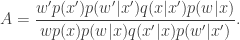

 , but the marginal for
