estimate – Darren Wilkinson's blog

Several papers have appeared recently discussing the issue of how to tune the number of particles used in the particle filter within a particle MCMC algorithm such as particle marginal Metropolis Hastings (PMMH). Three such papers are:

Doucet, Arnaud, Michael Pitt, and Robert Kohn. Efficient implementation of Markov chain Monte Carlo when using an unbiased likelihood estimator. arXiv preprint arXiv:1210.1871 (2012).
Pitt, Michael K., Ralph dos Santos Silva, Paolo Giordani, and Robert Kohn. On some properties of Markov chain Monte Carlo simulation methods based on the particle filter. Journal of Econometrics 171, no. 2 (2012): 134-151.
Sherlock, Chris, Alexandre H. Thiery, Gareth O. Roberts, and Jeffrey S. Rosenthal. On the efficiency of pseudo-marginal random walk Metropolis algorithms. arXiv preprint arXiv:1309.7209 (2013).

I have discussed psuedo marginal MCMC and particle MCMC algorithms in previous posts. It will be useful to refer back to these posts if these topics are unfamiliar. Within particle MCMC algorithms (and psuedo-marginal MCMC algorithms, more generally), an unbiased estimate of marginal likelihood is constructed using a number of particles. The more particles that are used, the better the estimate of marginal likelihood is, and the resulting MCMC algorithm will behave more like a “real” marginal MCMC algorithm. For a small number of particles, the algorithm will still have exactly the correct target, but the noise in the unbiased estimator of marginal likelihood will lead to poor mixing of the MCMC chain. The idea is to use just enough particles to ensure that there isn’t “too much” noise in the unbiased estimator, but not to waste lots of time producing a super-accurate estimate of marginal likelihood if that isn’t necessary to ensure good mixing of the MCMC chain.

The papers above try to give theoretical justifications for certain “rules of thumb” that are commonly used in practice. One widely adopted scheme is to tune the number of particles so that the variance of the log of the estimate of marginal liklihood is around one. The obvious questions are “where?” and “why?”, and these questions turn out to be connected. As we will see, there isn’t really a good answer to the “where?” question, but what people usually do is use a pilot run to get an estimate of the posterior mean, or mode, or MLE, and then pick one and tune the noise variance at that particular parameter value. As to “why?”, well, the papers above make various (slightly different) assumptions, all of which lead to trading off mixing against computation time to obtain an “optimal” number of particles. They don’t all agree that the variance of the noise should be exactly 1, but they all agree to an order of magnitude.

All of the above papers make the assumption that the noise distribution associated with the marginal likelihood estimate is independent of the parameter at which it is being evaluated, which explains why there isn’t a really good answer to the “where?” question – under the assumption it doesn’t matter what parameter value is used for tuning – they are all the same! Easy. Except that’s quite a big assumption, so it would be nice to know that it is reasonable, and unfortunately it isn’t. Let’s look at an example to see what goes wrong.

Example

In Chapter 10 of my book I look in detail at constructing a PMMH algorithm for inferring the parameters of a discretely observed stochastic Lotka-Volterra model. I’ve stepped through the computational details in a previous post which you should refer back to for the necessary background. Following that post, we can construct a particle filter to return an unbiased estimate of marginal likelihood using the following R code (which relies on the smfsb CRAN package):

require(smfsb)
# data
data(LVdata)
data=as.timedData(LVnoise10)
noiseSD=10
# measurement error model
dataLik <- function(x,t,y,log=TRUE,...)
{
    ll=sum(dnorm(y,x,noiseSD,log=TRUE))
    if (log)
        return(ll)
    else
        return(exp(ll))
}
# now define a sampler for the prior on the initial state
simx0 <- function(N,t0,...)
{
    mat=cbind(rpois(N,50),rpois(N,100))
    colnames(mat)=c("x1","x2")
    mat
}
# construct particle filter
mLLik=pfMLLik(150,simx0,0,stepLVc,dataLik,data)

Again, see the relevant previous post for details. So now mLLik() is a function that will return the log of an unbiased estimate of marginal likelihood (based on 150 particles) given a parameter value at which to evaluate.

What we are currently wondering is whether the noise in the estimate is independent of the parameter at which it is evaluated. We can investigate this for this filter easily by looking at how the estimate varies as the first parameter (prey birth rate) varies. The following code computes a log likelihood estimate across a range of values and plots the result.

mLLik1=function(x){mLLik(th=c(th1=x,th2=0.005,th3=0.6))}
x=seq(0.7,1.3,length.out=5001)
y=sapply(x,mLLik1)
plot(x[y>-1e10],y[y>-1e10])

The resulting plot is as follows (click for full size):

So, looking at the plot, it is very clear that the noise variance certainly isn’t constant as the parameter varies – it varies substantially. Furthermore, the way in which it varies is “dangerous”, in that the noise is smallest in the vicinity of the MLE. So, if a parameter close to the MLE is chosen for tuning the number of particles, this will ensure that the noise is small close to the MLE, but not elsewhere in parameter space. This could have bad consequences for the mixing of the MCMC algorithm as it explores the tails of the posterior distribution.

So with the above in mind, how should one tune the number of particles in a pMCMC algorithm? I can’t give a general answer, but I can explain what I do. We can’t rely on theory, so a pragmatic approach is required. The above rule of thumb usually gives a good starting point for exploration. Then I just directly optimise ESS per CPU second of the pMCMC algorithm from pilot runs for varying numbers of particles (and other tuning parameters in the algorithm). ESS is “expected sample size”, which can be estimated using the effectiveSize() function in the coda CRAN package. Ugly and brutish, but it works…

The pseudo-marginal approach to MCMC for Bayesian inference

In a previous post I described a generalisation of the Metropolis Hastings MCMC algorithm which uses unbiased Monte Carlo estimates of likelihood in the acceptance ratio, but is nevertheless exact, when considered as a pseudo-marginal approach to “exact approximate” MCMC. To be useful in the context of Bayesian inference, we need to be able to compute unbiased estimates of the (marginal) likelihood of the data given some proposed model parameters with any “latent variables” integrated out.

To be more precise, consider a model for data $y$ with parameters $\theta$ of the form $\pi(y|\theta)$ together with a prior on $\theta$ , $\pi(\theta)$ , giving a joint model

$\displaystyle \pi(\theta,y)=\pi(\theta)\pi(y|\theta).$

Suppose now that interest is in the posterior distribution

$\displaystyle \pi(\theta|y) \propto \pi(\theta,y)=\pi(\theta)\pi(y|\theta).$

We can construct a fairly generic (marginal) MCMC scheme for this posterior by first proposing $\theta^\star \sim f(\theta^\star|\theta)$ from some fairly arbitrary proposal distribution and then accepting the value with probability $\min\{1,A\}$ where

$\displaystyle A = \frac{\pi(\theta^\star)}{\pi(\theta)} \frac{f(\theta|\theta^\star)}{f(\theta^\star|\theta)} \frac{\pi(y|\theta^\star)}{\pi(y|\theta)}$

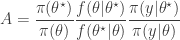
This method is great provided that the (marginal) likelihood of the data $\pi(y|\theta)$ is available to us analytically, but in many (most) interesting models it is not. However, in the previous post I explained why substituting in a Monte Carlo estimate $\hat\pi(y|\theta)$ will still lead to the exact posterior if the estimate is unbiased in the sense that $E[\hat\pi(y|\theta)]=\pi(y|\theta)$ . Consequently, sources of (cheap) unbiased Monte Carlo estimates of (marginal) likelihood are of potential interest in the development of exact MCMC algorithms.

Latent variables and marginalisation

Often the reason that we cannot evaluate $\pi(y|\theta)$ is that there are latent variables in the problem, and the model for the data is conditional on those latent variables. Explicitly, if we denote the latent variables by $x$ , then the joint distribution for the model takes the form

$\displaystyle \pi(\theta,x,y) = \pi(\theta)\pi(x|\theta)\pi(y|x,\theta)$

Now since

$\displaystyle \pi(y|\theta) = \int_X \pi(y|x,\theta)\pi(x|\theta)\,dx$

there is a simple and obvious Monte Carlo strategy for estimating $\pi(y|\theta)$ provided that we can evaluate $\pi(y|x,\theta)$ and simulate realisations from $\pi(x|\theta)$ . That is, simulate values $x_1,x_2,\ldots,x_n$ from $\pi(x|\theta)$ for some suitably large $n$ , and then put

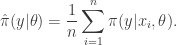
$\displaystyle \hat\pi(y|\theta) = \frac{1}{n}\sum_{i=1}^n \pi(y|x_i,\theta).$

It is clear by the law of large numbers that this estimate will converge to $\pi(y|\theta)$ as $n\rightarrow \infty$ . That is, $\hat\pi(y|\theta)$ is a consistent estimate of $\pi(y|\theta)$ . However, a moment’s thought reveals that this estimate is not only consistent, but also unbiased, since each term in the sum has expectation $\pi(y|\theta)$ . This simple Monte Carlo estimate of likelihood can therefore be substituted into a Metropolis-Hastings acceptance ratio without affecting the (marginal) target distribution of the Markov chain. Note that this estimate of marginal likelihood is sometimes referred to as the Rao-Blackwellised estimate, due to its connection with the Rao-Blackwell theorem.

Importance sampling

Suppose now that we cannot sample values directly from $\pi(x|\theta)$ , but can sample instead from a distribution $\pi'(x|\theta)$ having the same support as $\pi(x|\theta)$ . We can then instead produce an importance sampling estimate for $\pi(y|\theta)$ by noting that

$\displaystyle \pi(y|\theta) = \int_X \pi(y|x,\theta)\frac{\pi(x|\theta)}{\pi'(x|\theta)}\pi'(x|\theta)\,dx.$

Consequently, samples $x_1,x_2,\ldots,x_n$ from $\pi'(x|\theta)$ can be used to construct the estimate

$\displaystyle \hat{\pi}(y|\theta) = \frac{1}{n}\sum_{i=1}^n \pi(y|x_i,\theta) \frac{\pi(x_i|\theta)}{\pi'(x_i|\theta)}$

which again is clearly both consistent and unbiased. This estimate is often written

$\displaystyle \hat{\pi}(y|\theta) = \frac{1}{n}\sum_{i=1}^n \pi(y|x_i,\theta) w_i$
where $w_i=\pi(x_i|\theta)/\pi'(x_i|\theta)$ . The weights, $w_i$ , are known as importance weights.

Importance resampling

An idea closely related to that of importance sampling is that of importance resampling where importance weights are used to resample a sample in order to equalise the weights, often prior to a further round of weighting and resampling. The basic idea is to generate an approximate sample from a target density $\pi(x)$ using values sampled from an auxiliary distribution $\pi'(x)$ , where we now supress any dependence of the distributions on model parameters, $\theta$ .

First generate a sample $x_1,\ldots,x_n$ from $\pi'(x)$ and compute weights $w_i=\pi(x_i)/\pi'(x_i),\ i=1,\ldots,n$ . Then compute normalised weights $\tilde{w}_i=w_i/\sum_{k=1}^n w_k$ . Generate a new sample of size $n$ by sampling $n$ times with replacement from the original sample with the probability of choosing each value determined by its normalised weight.

As an example, consider using a sample from the Cauchy distribution as an auxiliary distribution for approximately sampling standard normal random quantities. We can do this using a few lines of R as follows.

n=1000
xa=rcauchy(n)
w=dnorm(xa)/dcauchy(xa)
x=sample(xa,n,prob=w,replace=TRUE)
hist(x,30)
mean(w)

Note that we don’t actually need to compute the normalised weights, as the sample function will do this for us. Note also that the average weight will be close to one. It should be clear that the expected value of the weights will be exactly 1 when both the target and auxiliary densities are correctly normalised. Also note that the procedure can be used when one or both of the densities are not correctly normalised, since the weights will be normalised prior to sampling anyway. Note that in this case the expected weight will be the (ratio of) normalising constant(s), and so looking at the average weight will give an estimate of the normalising constant.

Note that the importance sampling procedure is approximate. Unlike a technique such as rejection sampling, which leads to samples having exactly the correct distribution, this is not the case here. Indeed, it is clear that in the $n=1$ case, the final sample will be exactly drawn from the auxiliary and not the target. The procedure is asymptotic, in that it improves as the sample size increases, tending to the exact target as $n\rightarrow \infty$ .

We can understand why importance resampling works by first considering the univariate case, using correctly normalised densities. Consider a very large number of particles, $N$ . The proportion of the auxiliary samples falling in a small interval $[x,x+dx)$ will be $\pi'(x)dx$ , corresponding to roughly $N\pi'(x)dx$ particles. The weight for each of those particles will be $w(x)=\pi(x)/\pi'(x)$ , and since the expected weight of a random particle is 1, the sum of all weights will be (roughly) $N$ , leading to normalised weights for the particles near $x$ of $\tilde{w}(x)=\pi(x)/[N\pi'(x)]$ . The combined weight of all particles in $[x,x+dx)$ is therefore $\pi(x)dx$ . Clearly then, when we resample $N$ times we expect to select roughly $N\pi(x)dx$ particles from this interval. This corresponds to a proportion $\pi(x)dt$ , corresponding to a density of $\pi(x)$ in the final sample.

Obviously the above argument is very informal, but can be tightened up into a reasonably rigorous proof for the 1d case without too much effort, and the multivariate extension is also reasonably clear.

The bootstrap particle filter

The bootstrap particle filter is an iterative method for carrying out Bayesian inference for dynamic state space (partially observed Markov process) models, sometimes also known as hidden Markov models (HMMs). Here, an unobserved Markov process, $x_0,x_1,\ldots,x_T$ governed by a transition kernel $p(x_{t+1}|x_t)$ is partially observed via some measurement model $p(y_t|x_t)$ leading to data $y_1,\ldots,y_T$ . The idea is to make inference for the hidden states $x_{0:T}$ given the data $y_{1:T}$ . The method is a very simple application of the importance resampling technique. At each time, $t$ , we assume that we have a (approximate) sample from $p(x_t|y_{1:t})$ and use importance resampling to generate an approximate sample from $p(x_{t+1}|y_{1:t+1})$ .

More precisely, the procedure is initialised with a sample from $x_0^k \sim p(x_0),\ k=1,\ldots,M$ with uniform normalised weights ${w'}_0^k=1/M$ . Then suppose that we have a weighted sample $\{x_t^k,{w'}_t^k|k=1,\ldots,M\}$ from $p(x_t|y_{1:t})$ . First generate an equally weighted sample by resampling with replacement $M$ times to obtain $\{\tilde{x}_t^k|k=1,\ldots,M\}$ (giving an approximate random sample from $p(x_t|y_{1:t})$ ). Note that each sample is independently drawn from $\sum_{i=1}^M {w'}_t^i\delta(x-x_t^i)$ . Next propagate each particle forward according to the Markov process model by sampling $x_{t+1}^k\sim p(x_{t+1}|\tilde{x}_t^k),\ k=1,\ldots,M$ (giving an approximate random sample from $p(x_{t+1}|y_{1:t})$ ). Then for each of the new particles, compute a weight $w_{t+1}^k=p(y_{t+1}|x_{t+1}^k)$ , and then a normalised weight ${w'}_{t+1}^k=w_{t+1}^k/\sum_i w_{t+1}^i$ .

It is clear from our understanding of importance resampling that these weights are appropriate for representing a sample from $p(x_{t+1}|y_{1:t+1})$ , and so the particles and weights can be propagated forward to the next time point. It is also clear that the average weight at each time gives an estimate of the marginal likelihood of the current data point given the data so far. So we define

$\displaystyle \hat{p}(y_t|y_{1:t-1})=\frac{1}{M}\sum_{k=1}^M w_t^k$

and

$\displaystyle \hat{p}(y_{1:T}) = \hat{p}(y_1)\prod_{t=2}^T \hat{p}(y_t|y_{1:t-1}).$

Again, from our understanding of importance resampling, it should be reasonably clear that $\hat{p}(y_{1:T})$ is a consistent estimator of ${p}(y_{1:T})$ . It is much less clear, but nevertheless true that this estimator is also unbiased. The standard reference for this fact is Del Moral (2004), but this is a rather technical monograph. A much more accessible proof (for a very general particle filter) is given in Pitt et al (2011).

It should therefore be clear that if one is interested in developing MCMC algorithms for state space models, one can use a pseudo-marginal MCMC scheme, substituting in $\hat{p}_\theta(y_{1:T})$ from a bootstrap particle filter in place of $p(y_{1:T}|\theta)$ . This turns out to be a simple special case of the particle marginal Metropolis-Hastings (PMMH) algorithm described in Andreiu et al (2010). However, the PMMH algorithm in fact has the full joint posterior $p(\theta,x_{0:T}|y_{1:T})$ as its target. I will explain the PMMH algorithm in a subsequent post.

Tag: estimate

Tuning particle MCMC algorithms