Comonads for scientific and statistical computing in Scala

Introduction

In a previous post I’ve given a brief introduction to monads in Scala, aimed at people interested in scientific and statistical computing. Monads are a concept from category theory which turn out to be exceptionally useful for solving many problems in functional programming. But most categorical concepts have a dual, usually prefixed with “co”, so the dual of a monad is the comonad. Comonads turn out to be especially useful for formulating algorithms from scientific and statistical computing in an elegant way. In this post I’ll illustrate their use in signal processing, image processing, numerical integration of PDEs, and Gibbs sampling (of an Ising model). Comonads enable the extension of a local computation to a global computation, and this pattern crops up all over the place in statistical computing.

Monads and comonads

Simplifying massively, from the viewpoint of a Scala programmer, a monad is a mappable (functor) type class augmented with the methods pure and flatMap:

trait Monad[M[_]] extends Functor[M] {
  def pure[T](v: T): M[T]
  def flatMap[T,S](v: M[T])(f: T => M[S]): M[S]
}

In category theory, the dual of a concept is typically obtained by “reversing the arrows”. Here that means reversing the direction of the methods pure and flatMap to get extract and coflatMap, respectively.

trait Comonad[W[_]] extends Functor[W] {
  def extract[T](v: W[T]): T
  def coflatMap[T,S](v: W[T])(f: W[T] => S): W[S]
}

So, while pure allows you to wrap plain values in a monad, extract allows you to get a value out of a comonad. So you can always get a value out of a comonad (unlike a monad). Similarly, while flatMap allows you to transform a monad using a function returning a monad, coflatMap allows you to transform a comonad using a function which collapses a comonad to a single value. It is coflatMap (sometimes called extend) which can extend a local computation (producing a single value) to the entire comonad. We’ll look at how that works in the context of some familiar examples.

Applying a linear filter to a data stream

One of the simplest examples of a comonad is an infinite stream of data. I’ve discussed streams in a previous post. By focusing on infinite streams we know the stream will never be empty, so there will always be a value that we can extract. Which value does extract give? For a Stream encoded as some kind of lazy list, the only value we actually know is the value at the head of the stream, with subsequent values to be lazily computed as required. So the head of the list is the only reasonable value for extract to return.

Understanding coflatMap is a bit more tricky, but it is coflatMap that provides us with the power to apply a non-trivial statistical computation to the stream. The input is a function which transforms a stream into a value. In our example, that will be a function which computes a weighted average of the first few values and returns that weighted average as the result. But the return type of coflatMap must be a stream of such computations. Following the types, a few minutes thought reveals that the only reasonable thing to do is to return the stream formed by applying the weighted average function to all sub-streams, recursively. So, for a Stream s (of type Stream[T]) and an input function f: W[T] => S, we form a stream whose head is f(s) and whose tail is coflatMap(f) applied to s.tail. Again, since we are working with an infinite stream, we don’t have to worry about whether or not the tail is empty. This gives us our comonadic Stream, and it is exactly what we need for applying a linear filter to the data stream.

In Scala, Cats is a library providing type classes from Category theory, and instances of those type classes for parametrised types in the standard library. In particular, it provides us with comonadic functionality for the standard Scala Stream. Let’s start by defining a stream corresponding to the logistic map.

import cats._
import cats.implicits._

val lam = 3.7
def s = Stream.iterate(0.5)(x => lam*x*(1-x))
s.take(10).toList
// res0: List[Double] = List(0.5, 0.925, 0.25668749999999985,
//  0.7059564011718747, 0.7680532550204203, 0.6591455741499428, ...

Let us now suppose that we want to apply a linear filter to this stream, in order to smooth the values. The idea behind using comonads is that you figure out how to generate one desired value, and let coflatMap take care of applying the same logic to the rest of the structure. So here, we need a function to generate the first filtered value (since extract is focused on the head of the stream). A simple first attempt a function to do this might look like the following.

  def linearFilterS(weights: Stream[Double])(s: Stream[Double]): Double =
    (weights, s).parMapN(_*_).sum

This aligns each weight in parallel with a corresponding value from the stream, and combines them using multiplication. The resulting (hopefully finite length) stream is then summed (with addition). We can test this with

linearFilterS(Stream(0.25,0.5,0.25))(s)
// res1: Double = 0.651671875

and let coflatMap extend this computation to the rest of the stream with something like:

s.coflatMap(linearFilterS(Stream(0.25,0.5,0.25))).take(5).toList
// res2: List[Double] = List(0.651671875, 0.5360828502929686, ...

This is all completely fine, but our linearFilterS function is specific to the Stream comonad, despite the fact that all we’ve used about it in the function is that it is a parallelly composable and foldable. We can make this much more generic as follows:

  def linearFilter[F[_]: Foldable, G[_]](
    weights: F[Double], s: F[Double]
  )(implicit ev: NonEmptyParallel[F, G]): Double =
    (weights, s).parMapN(_*_).fold

This uses some fairly advanced Scala concepts which I don’t want to get into right now (I should also acknowledge that I had trouble getting the syntax right for this, and got help from Fabio Labella (@SystemFw) on the Cats gitter channel). But this version is more generic, and can be used to linearly filter other data structures than Stream. We can use this for regular Streams as follows:

s.coflatMap(s => linearFilter(Stream(0.25,0.5,0.25),s))
// res3: scala.collection.immutable.Stream[Double] = Stream(0.651671875, ?)

But we can apply this new filter to other collections. This could be other, more sophisticated, streams such as provided by FS2, Monix or Akka streams. But it could also be a non-stream collection, such as List:

val sl = s.take(10).toList
sl.coflatMap(sl => linearFilter(List(0.25,0.5,0.25),sl))
// res4: List[Double] = List(0.651671875, 0.5360828502929686, ...

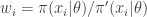
Assuming that we have the Breeze scientific library available, we can plot the raw and smoothed trajectories.

def myFilter(s: Stream[Double]): Double =
  linearFilter(Stream(0.25, 0.5, 0.25),s)
val n = 500
import breeze.plot._
import breeze.linalg._
val fig = Figure(s"The (smoothed) logistic map (lambda=$lam)")
val p0 = fig.subplot(3,1,0)
p0 += plot(linspace(1,n,n),s.take(n))
p0.ylim = (0.0,1.0)
p0.title = s"The logistic map (lambda=$lam)"
val p1 = fig.subplot(3,1,1)
p1 += plot(linspace(1,n,n),s.coflatMap(myFilter).take(n))
p1.ylim = (0.0,1.0)
p1.title = "Smoothed by a simple linear filter"
val p2 = fig.subplot(3,1,2)
p2 += plot(linspace(1,n,n),s.coflatMap(myFilter).coflatMap(myFilter).coflatMap(myFilter).coflatMap(myFilter).coflatMap(myFilter).take(n))
p2.ylim = (0.0,1.0)
p2.title = "Smoothed with 5 applications of the linear filter"
fig.refresh

Image processing and the heat equation

Streaming data is in no way the only context in which a comonadic approach facilitates an elegant approach to scientific and statistical computing. Comonads crop up anywhere where we want to extend a computation that is local to a small part of a data structure to the full data structure. Another commonly cited area of application of comonadic approaches is image processing (I should acknowledge that this section of the post is very much influenced by a blog post on comonadic image processing in Haskell). However, the kinds of operations used in image processing are in many cases very similar to the operations used in finite difference approaches to numerical integration of partial differential equations (PDEs) such as the heat equation, so in this section I will blur (sic) the distinction between the two, and numerically integrate the 2D heat equation in order to Gaussian blur a noisy image.

First we need a simple image type which can have pixels of arbitrary type T (this is very important – all functors must be fully type polymorphic).

  import scala.collection.parallel.immutable.ParVector
  case class Image[T](w: Int, h: Int, data: ParVector[T]) {
    def apply(x: Int, y: Int): T = data(x*h+y)
    def map[S](f: T => S): Image[S] = Image(w, h, data map f)
    def updated(x: Int, y: Int, value: T): Image[T] =
      Image(w,h,data.updated(x*h+y,value))
  }

Here I’ve chosen to back the image with a parallel immutable vector. This wasn’t necessary, but since this type has a map operation which automatically parallelises over multiple cores, any map operations applied to the image will be automatically parallelised. This will ultimately lead to all of our statistical computations being automatically parallelised without us having to think about it.

As it stands, this image isn’t comonadic, since it doesn’t implement extract or coflatMap. Unlike the case of Stream, there isn’t really a uniquely privileged pixel, so it’s not clear what extract should return. For many data structures of this type, we make them comonadic by adding a “cursor” pointing to a “current” element of interest, and use this as the focus for computations applied with coflatMap. This is simplest to explain by example. We can define our “pointed” image type as follows:

  case class PImage[T](x: Int, y: Int, image: Image[T]) {
    def extract: T = image(x, y)
    def map[S](f: T => S): PImage[S] = PImage(x, y, image map f)
    def coflatMap[S](f: PImage[T] => S): PImage[S] = PImage(
      x, y, Image(image.w, image.h,
      (0 until (image.w * image.h)).toVector.par.map(i => {
        val xx = i / image.h
        val yy = i % image.h
        f(PImage(xx, yy, image))
      })))

There is missing a closing brace, as I’m not quite finished. Here x and y represent the location of our cursor, so extract returns the value of the pixel indexed by our cursor. Similarly, coflatMap forms an image where the value of the image at each location is the result of applying the function f to the image which had the cursor set to that location. Clearly f should use the cursor in some way, otherwise the image will have the same value at every pixel location. Note that map and coflatMap operations will be automatically parallelised. The intuitive idea behind coflatMap is that it extends local computations. For the stream example, the local computation was a linear combination of nearby values. Similarly, in image analysis problems, we often want to apply a linear filter to nearby pixels. We can get at the pixel at the cursor location using extract, but we probably also want to be able to move the cursor around to nearby locations. We can do that by adding some appropriate methods to complete the class definition.

    def up: PImage[T] = {
      val py = y-1
      val ny = if (py >= 0) py else (py + image.h)
      PImage(x,ny,image)
    }
    def down: PImage[T] = {
      val py = y+1
      val ny = if (py < image.h) py else (py - image.h)
      PImage(x,ny,image)
    }
    def left: PImage[T] = {
      val px = x-1
      val nx = if (px >= 0) px else (px + image.w)
      PImage(nx,y,image)
    }
    def right: PImage[T] = {
      val px = x+1
      val nx = if (px < image.w) px else (px - image.w)
      PImage(nx,y,image)
    }
  }

Here each method returns a new pointed image with the cursor shifted by one pixel in the appropriate direction. Note that I’ve used periodic boundary conditions here, which often makes sense for numerical integration of PDEs, but makes less sense for real image analysis problems. Note that we have embedded all “indexing” issues inside the definition of our classes. Now that we have it, none of the statistical algorithms that we develop will involve any explicit indexing. This makes it much less likely to develop algorithms containing bugs corresponding to “off-by-one” or flipped axis errors.

This class is now fine for our requirements. But if we wanted Cats to understand that this structure is really a comonad (perhaps because we wanted to use derived methods, such as coflatten), we would need to provide evidence for this. The details aren’t especially important for this post, but we can do it simply as follows:

  implicit val pimageComonad = new Comonad[PImage] {
    def extract[A](wa: PImage[A]) = wa.extract
    def coflatMap[A,B](wa: PImage[A])(f: PImage[A] => B): PImage[B] =
      wa.coflatMap(f)
    def map[A,B](wa: PImage[A])(f: A => B): PImage[B] = wa.map(f)
  }

It’s handy to have some functions for converting Breeze dense matrices back and forth with our image class.

  import breeze.linalg.{Vector => BVec, _}
  def BDM2I[T](m: DenseMatrix[T]): Image[T] =
    Image(m.cols, m.rows, m.data.toVector.par)
  def I2BDM(im: Image[Double]): DenseMatrix[Double] =
    new DenseMatrix(im.h,im.w,im.data.toArray)

Now we are ready to see how to use this in practice. Let’s start by defining a very simple linear filter.

def fil(pi: PImage[Double]): Double = (2*pi.extract+
  pi.up.extract+pi.down.extract+pi.left.extract+pi.right.extract)/6.0

This simple filter can be used to “smooth” or “blur” an image. However, from a more sophisticated viewpoint, exactly this type of filter can be used to represent one time step of a numerical method for time integration of the 2D heat equation. Now we can simulate a noisy image and apply our filter to it using coflatMap:

import breeze.stats.distributions.Gaussian
val bdm = DenseMatrix.tabulate(200,250){case (i,j) => math.cos(
  0.1*math.sqrt((i*i+j*j))) + Gaussian(0.0,2.0).draw}
val pim0 = PImage(0,0,BDM2I(bdm))
def pims = Stream.iterate(pim0)(_.coflatMap(fil))

Note that here, rather than just applying the filter once, I’ve generated an infinite stream of pointed images, each one representing an additional application of the linear filter. Thus the sequence represents the time solution of the heat equation with initial condition corresponding to our simulated noisy image.

We can render the first few frames to check that it seems to be working.

import breeze.plot._
val fig = Figure("Diffusing a noisy image")
pims.take(25).zipWithIndex.foreach{case (pim,i) => {
  val p = fig.subplot(5,5,i)
  p += image(I2BDM(pim.image))
}}

Note that the numerical integration is carried out in parallel on all available cores automatically. Other image filters can be applied, and other (parabolic) PDEs can be numerically integrated in an essentially similar way.

Gibbs sampling the Ising model

Another place where the concept of extending a local computation to a global computation crops up is in the context of Gibbs sampling a high-dimensional probability distribution by cycling through the sampling of each variable in turn from its full-conditional distribution. I’ll illustrate this here using the Ising model, so that I can reuse the pointed image class from above, but the principles apply to any Gibbs sampling problem. In particular, the Ising model that we consider has a conditional independence structure corresponding to a graph of a square lattice. As above, we will use the comonadic structure of the square lattice to construct a Gibbs sampler. However, we can construct a Gibbs sampler for arbitrary graphical models in an essentially identical way by using a graph comonad.

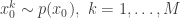
Let’s begin by simulating a random image containing +/-1s:

import breeze.stats.distributions.{Binomial,Bernoulli}
val beta = 0.4
val bdm = DenseMatrix.tabulate(500,600){
  case (i,j) => (new Binomial(1,0.2)).draw
}.map(_*2 - 1) // random matrix of +/-1s
val pim0 = PImage(0,0,BDM2I(bdm))

We can use this to initialise our Gibbs sampler. We now need a Gibbs kernel representing the update of each pixel.

def gibbsKernel(pi: PImage[Int]): Int = {
   val sum = pi.up.extract+pi.down.extract+pi.left.extract+pi.right.extract
   val p1 = math.exp(beta*sum)
   val p2 = math.exp(-beta*sum)
   val probplus = p1/(p1+p2)
   if (new Bernoulli(probplus).draw) 1 else -1
}

So far so good, but there a couple of issues that we need to consider before we plough ahead and start coflatMapping. The first is that pure functional programmers will object to the fact that this function is not pure. It is a stochastic function which has the side-effect of mutating the random number state. I’m just going to duck that issue here, as I’ve previously discussed how to fix it using probability monads, and I don’t want it to distract us here.

However, there is a more fundamental problem here relating to parallel versus sequential application of Gibbs kernels. coflatMap is conceptually parallel (irrespective of how it is implemented) in that all computations used to build the new comonad are based solely on the information available in the starting comonad. OTOH, detailed balance of the Markov chain will only be preserved if the kernels for each pixel are applied sequentially. So if we coflatMap this kernel over the image we will break detailed balance. I should emphasise that this has nothing to do with the fact that I’ve implemented the pointed image using a parallel vector. Exactly the same issue would arise if we switched to backing the image with a regular (sequential) immutable Vector.

The trick here is to recognise that if we coloured alternate pixels black and white using a chequerboard pattern, then all of the black pixels are conditionally independent given the white pixels and vice-versa. Conditionally independent pixels can be updated by parallel application of a Gibbs kernel. So we just need separate kernels for updating odd and even pixels.

def oddKernel(pi: PImage[Int]): Int =
  if ((pi.x+pi.y) % 2 != 0) pi.extract else gibbsKernel(pi)
def evenKernel(pi: PImage[Int]): Int =
  if ((pi.x+pi.y) % 2 == 0) pi.extract else gibbsKernel(pi)

Each of these kernels can be coflatMapped over the image preserving detailed balance of the chain. So we can now construct an infinite stream of MCMC iterations as follows.

def pims = Stream.iterate(pim0)(_.coflatMap(oddKernel).
  coflatMap(evenKernel))

We can animate the first few iterations with:

import breeze.plot._
val fig = Figure("Ising model Gibbs sampler")
fig.width = 1000
fig.height = 800
pims.take(50).zipWithIndex.foreach{case (pim,i) => {
  print(s"$i ")
  fig.clear
  val p = fig.subplot(1,1,0)
  p.title = s"Ising model: frame $i"
  p += image(I2BDM(pim.image.map{_.toDouble}))
  fig.refresh
}}
println

Here I have a movie showing the first 1000 iterations. Note that youtube seems to have over-compressed it, but you should get the basic idea.

Again, note that this MCMC sampler runs in parallel on all available cores, automatically. This issue of odd/even pixel updating emphasises another issue that crops up a lot in functional programming: very often, thinking about how to express an algorithm functionally leads to an algorithm which parallelises naturally. For general graphs, figuring out which groups of nodes can be updated in parallel is essentially the graph colouring problem. I’ve discussed this previously in relation to parallel MCMC in:

Wilkinson, D. J. (2005) Parallel Bayesian Computation, Chapter 16 in E. J. Kontoghiorghes (ed.) Handbook of Parallel Computing and Statistics, Marcel Dekker/CRC Press, 481-512.

Further reading

There are quite a few blog posts discussing comonads in the context of Haskell. In particular, the post on comonads for image analysis I mentioned previously, and this one on cellular automata. Bartosz’s post on comonads gives some connection back to the mathematical origins. Runar’s Scala comonad tutorial is the best source I know for comonads in Scala.

Full runnable code corresponding to this blog post is available from my blog repo.

Calling Scala code from R using jvmr

[Update: the jvmr package has been replaced by a new package called rscala. I have a new post which explains it.]

Introduction

In previous posts I have explained why I think that Scala is a good language to use for statistical computing and data science. Despite this, R is very convenient for simple exploratory data analysis and visualisation – currently more convenient than Scala. I explained in my recent talk at the RSS what (relatively straightforward) things would need to be developed for Scala in order to make R completely redundant, but for the short term at least, it seems likely that I will need to use both R and Scala for my day-to-day work.

Since I use both Scala and R for statistical computing, it is very convenient to have a degree of interoperability between the two languages. I could call R from Scala code or Scala from R code, or both. Fortunately, some software tools have been developed recently which make this much simpler than it used to be. The software is jvmr, and as explained at the website, it enables calling Java and Scala from R and calling R from Java and Scala. I have previously discussed calling Java from R using the R CRAN package rJava. In this post I will focus on calling Scala from R using the CRAN package jvmr, which depends on rJava. I may examine calling R from Scala in a future post.

On a system with Java installed, it should be possible to install the jvmr R package with a simple

install.packages("jvmr")

from the R command prompt. The package has the usual documentation associated with it, but the draft paper describing the package is the best way to get an overview of its capabilities and a walk-through of simple usage.

A Gibbs sampler in Scala using Breeze

For illustration I’m going to use a Scala implementation of a Gibbs sampler which relies on the Breeze scientific library, and will be built using the simple build tool, sbt. Most non-trivial Scala projects depend on various versions of external libraries, and sbt is an easy way to build even very complex projects trivially on any system with Java installed. You don’t even need to have Scala installed in order to build and run projects using sbt. I give some simple complete worked examples of building and running Scala sbt projects in the github repo associated with my recent RSS talk. Installing sbt is trivial as explained in the repo READMEs.

For this post, the Scala code, gibbs.scala is given below:

package gibbs

object Gibbs {

    import scala.annotation.tailrec
    import scala.math.sqrt
    import breeze.stats.distributions.{Gamma,Gaussian}

    case class State(x: Double, y: Double) {
      override def toString: String = x.toString + " , " + y + "\n"
    }

    def nextIter(s: State): State = {
      val newX = Gamma(3.0, 1.0/((s.y)*(s.y)+4.0)).draw
      State(newX, Gaussian(1.0/(newX+1), 1.0/sqrt(2*newX+2)).draw)
    }

    @tailrec def nextThinnedIter(s: State,left: Int): State =
      if (left==0) s else nextThinnedIter(nextIter(s),left-1)

    def genIters(s: State, stop: Int, thin: Int): List[State] = {
      @tailrec def go(s: State, left: Int, acc: List[State]): List[State] =
        if (left>0)
          go(nextThinnedIter(s,thin), left-1, s::acc)
          else acc
      go(s,stop,Nil).reverse
    }

    def main(args: Array[String]) = {
      if (args.length != 3) {
        println("Usage: sbt \"run <outFile> <iters> <thin>\"")
        sys.exit(1)
      } else {
        val outF=args(0)
        val iters=args(1).toInt
        val thin=args(2).toInt
        val out = genIters(State(0.0,0.0),iters,thin)
        val s = new java.io.FileWriter(outF)
        s.write("x , y\n")
        out map { it => s.write(it.toString) }
        s.close
      }
    }

}

This code requires Scala and the Breeze scientific library in order to build. We can specify this in a sbt build file, which should be called build.sbt and placed in the same directory as the Scala code.

name := "gibbs"

version := "0.1"

scalacOptions ++= Seq("-unchecked", "-deprecation", "-feature")

libraryDependencies  ++= Seq(
            "org.scalanlp" %% "breeze" % "0.10",
            "org.scalanlp" %% "breeze-natives" % "0.10"
)

resolvers ++= Seq(
            "Sonatype Snapshots" at "https://oss.sonatype.org/content/repositories/snapshots/",
            "Sonatype Releases" at "https://oss.sonatype.org/content/repositories/releases/"
)

scalaVersion := "2.11.2"

Now, from a system command prompt in the directory where the files are situated, it should be possible to download all dependencies and compile and run the code with a simple

sbt "run output.csv 50000 1000"

Calling via R system calls

Since this code takes a relatively long time to run, calling it from R via simple system calls isn’t a particularly terrible idea. For example, we can do this from the R command prompt with the following commands

system("sbt \"run output.csv 50000 1000\"")
out=read.csv("output.csv")
library(smfsb)
mcmcSummary(out,rows=2)

This works fine, but won’t work so well for code which needs to be called repeatedly. For this, tighter integration between R and Scala would be useful, which is where jvmr comes in.

Calling sbt-based Scala projects via jvmr

jvmr provides a very simple way to embed a Scala interpreter within an R session, to be able to execute Scala expressions from R and to have the results returned back to the R session for further processing. The main issue with using this in practice is managing dependencies on external libraries and setting the Scala classpath correctly. For an sbt project such as we are considering here, it is relatively easy to get sbt to provide us with all of the information we need in a fully automated way.

First, we need to add a new task to our sbt build instructions, which will output the full classpath in a way that is easy to parse from R. Just add the following to the end of the file build.sbt:

lazy val printClasspath = taskKey[Unit]("Dump classpath")

printClasspath := {
  (fullClasspath in Runtime value) foreach {
    e => print(e.data+"!")
  }
}

Be aware that blank lines are significant in sbt build files. Once we have this in our build file, we can write a small R function to get the classpath from sbt and then initialise a jvmr scalaInterpreter with the correct full classpath needed for the project. An R function which does this, sbtInit(), is given below

sbtInit<-function()
{
  library(jvmr)
  system2("sbt","compile")
  cpstr=system2("sbt","printClasspath",stdout=TRUE)
  cpst=cpstr[length(cpstr)]
  cpsp=strsplit(cpst,"!")[[1]]
  cp=cpsp[1:(length(cpsp)-1)]
  scalaInterpreter(cp,use.jvmr.class.path=FALSE)
}

With this function at our disposal, it becomes trivial to call our Scala code direct from the R interpreter, as the following code illustrates.

sc=sbtInit()
sc['import gibbs.Gibbs._']
out=sc['genIters(State(0.0,0.0),50000,1000).toArray.map{s=>Array(s.x,s.y)}']
library(smfsb)
mcmcSummary(out,rows=2)

Here we call the getIters function directly, rather than via the main method. This function returns an immutable List of States. Since R doesn’t understand this, we map it to an Array of Arrays, which R then unpacks into an R matrix for us to store in the matrix out.

Summary

The CRAN package jvmr makes it very easy to embed a Scala interpreter within an R session. However, for most non-trivial statistical computing problems, the Scala code will have dependence on external scientific libraries such as Breeze. The standard way to easily manage external dependencies in the Scala ecosystem is sbt. Given an sbt-based Scala project, it is easy to add a task to the sbt build file and a function to R in order to initialise the jvmr Scala interpreter with the full classpath needed to call arbitrary Scala functions. This provides very convenient inter-operability between R and Scala for many statistical computing applications.

Introduction to the particle Gibbs sampler

Introduction

Particle MCMC (the use of approximate SMC proposals within exact MCMC algorithms) is arguably one of the most important developments in computational Bayesian inference of the 21st Century. The key concepts underlying these methods are described in a famously impenetrable “read paper” by Andrieu et al (2010). Probably the most generally useful method outlined in that paper is the particle marginal Metropolis-Hastings (PMMH) algorithm that I have described previously – that post is required preparatory reading for this one.

In this post I want to discuss some of the other topics covered in the pMCMC paper, leading up to a description of the particle Gibbs sampler. The basic particle Gibbs algorithm is arguably less powerful than PMMH for a few reasons, some of which I will elaborate on. But there is still a lot of active research concerning particle Gibbs-type algorithms, which are attempting to address some of the deficiencies of the basic approach. Clearly, in order to understand and appreciate the recent developments it is first necessary to understand the basic principles, and so that is what I will concentrate on here. I’ll then finish with some pointers to more recent work in this area.

PIMH

I will adopt the same approach and notation as for my post on the PMMH algorithm, using a simple bootstrap particle filter for a state space model as the SMC proposal. 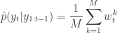It is simplest to understand particle Gibbs first in the context of known static parameters, and so it is helpful to first reconsider the special case of the PMMH algorithm where there are no unknown parameters and only the state path, of the process is being updated. That is, we target (for known, fixed, ) rather than . This special case is known as the particle independent Metropolis-Hastings (PIMH) sampler.

Here we envisage proposing a new path using a bootstrap filter, and then accepting the proposal with probability , where is the Metropolis-Hastings ratio

where is the bootstrap filter’s estimate of marginal likelihood for the new path, and is the estimate associated with the current path. Again using notation from the previous post it is clear that this ratio targets a distribution on the joint space of all simulated random variables proportional to

and that in this case the marginal distribution of the accepted path is exactly . Again, be sure to see the previous post for the explanation.

Conditional SMC update

So far we have just recapped the previous post in the case of known parameters, but it gives us insight in how to proceed. A general issue with Metropolis independence samplers in high dimensions is that they often exhibit “sticky” behaviour, whereby an unusually “good” accepted path is hard to displace. This motivates consideration of a block-Gibbs-style algorithm where updates are used that are always accepted. It is clear that simply running a bootstrap filter will target the particle filter distribution

and so the marginal distribution of the accepted path will be the approximate rather than the exact conditional distribution . However, we know from consideration of the PIMH algorithm that what we really want to do is target the slightly modified distribution proportional to

,

as this will lead to accepted paths with the exact marginal distribution. For the PIMH this modification is achieved using a Metropolis-Hastings correction, but we now try to avoid this by instead conditioning on the previously accepted path. For this target the accepted paths have exactly the required marginal distribution, so we now write the target as the product of the marginal for the current path times a conditional for all of the remaining variables.

where in addition to the correct marginal for we assume iid uniform ancestor indices. The important thing to note here is that the conditional distribution of the remaining variables simplifies to

.

The terms in the denominator are precisely the terms in the numerator corresponding to the current path, and hence “cancel out” the current path terms in the numerator. It is therefore clear that we can sample directly from this conditional distribution by running a bootstrap particle filter that includes the current path and which leaves the current path fixed. This is the conditional SMC (CSMC) update, which here is just a conditional bootstrap particle filter update. It is clear from the form of the conditional density how this filter must be constructed, but for completeness it is described below.

The bootstrap filter is run conditional on one trajectory. This is usually the trajectory sampled at the last run of the particle filter. The idea is that you do not sample new state or ancestor values for that one trajectory. Note that this guarantees that the conditioned on trajectory survives the filter right through to the final sweep of the filter at which point a new trajectory is picked from the current selection of paths, of which the conditioned-on trajectory is one.

Let be the path that is to be conditioned on, with ancestral lineage . Then, for , sample and set . Now suppose that at time we have a weighted sample from . First resample by sampling . Next sample . Then for all set and normalise with . Propagate this weighted set of particles to the next time point. At time select a single trajectory by sampling .

This defines a block Gibbs sampler which updates of the random variables in the augmented state space at each iteration. Since the block of variables to be updated is random, this defines an ergodic sampler for particles, and we have explained why the marginal distribution of the selected trajectory is the exact conditional distribution.

Before going on to consider the introduction of unknown parameters, it is worth considering the limitations of this method. One of the main motivations for considering a Gibbs-style update was concern about the “stickiness” of a Metropolis independence sampler. However, it is clear that conditional SMC updates also have the potential to stick. For a large number of time points, particle filter genealogies coalesce, or degenerate, to a single path. Since here we are conditioning on the current path, if there is coalescence, it is guaranteed to be to the previous path. So although the conditional SMC updates are always accepted, it is likely that much of the new path will be identical to the previous path, which is just another kind of “sticking” of the sampler. This problem with conditional SMC and particle Gibbs more generally is well recognised, and quite a bit of recent research activity in this area is directed at alleviating this sticking problem. The most obvious strategy to use is “backward sampling” (Godsill et al, 2004), which has been used in this context by Lindsten and Schon (2012), Whiteley et al (2010), and Chopin and Singh (2013), among others. Another related idea is “ancestor sampling” (Lindsten et al, 2014), which can be done in a single forward pass. Both of these techniques work well, but both rely on the tractability of the transition kernel of the state space model, which can be problematic in certain applications.

Particle Gibbs sampling

As we are working in the context of Gibbs-style updates, the introduction of static parameters, , into the problem is relatively straightforward. It turns out to be correct to do the obvious thing, which is to alternate between sampling given and the currently sampled path, , and sampling a new path using a conditional SMC update, conditional on the previous path in addition to and . Although this is the obvious thing to do, understanding exactly why it works is a little delicate, due to the augmented state space and conditional SMC update. However, it is reasonably clear that this strategy defines a “collapsed Gibbs sampler” (Lui, 1994), and so actually everything is fine. This particular collapsed Gibbs sampler is relatively easy to understand as a marginal sampler which integrates out the augmented variables, but then nevertheless samples the augmented variables at each iteration conditional on everything else.

Note that the Gibbs update of may be problematic in the context of a state space model with intractable transition kernel.

In a subsequent post I’ll show how to code up the particle Gibbs and other pMCMC algorithms in a reasonably efficient way.

References

• Andrieu, Christophe, Arnaud Doucet, and Roman Holenstein. “Particle Markov chain Monte Carlo methods.” Journal of the Royal Statistical Society: Series B (Statistical Methodology) 72.3 (2010): 269-342.
• Chopin, Nicolas, and Sumeetpal S. Singh. “On the particle Gibbs sampler.” arXiv preprint arXiv:1304.1887 (2013).
• Godsill, Simon J., Arnaud Doucet, and Mike West. “Monte Carlo smoothing for nonlinear time series.” Journal of the American Statistical Association 99.465 (2004).
• Lindsten, Fredrik, and Thomas B. Schön. “On the use of backward simulation in the particle Gibbs sampler.” Acoustics, Speech and Signal Processing (ICASSP), 2012 IEEE International Conference on. IEEE, 2012.
• Lindsten, Fredrik, Michael I. Jordan, and Thomas B. Schön. “Particle Gibbs with Ancestor Sampling.” arXiv preprint arXiv:1401.0604 (2014).
• Liu, Jun S. “The collapsed Gibbs sampler in Bayesian computations with applications to a gene regulation problem.” Journal of the American Statistical Association 89.427 (1994): 958-966.
• Whiteley, Nick, Christophe Andrieu, and Arnaud Doucet. “Efficient Bayesian inference for switching state-space models using discrete particle Markov chain Monte Carlo methods.” arXiv preprint arXiv:1011.2437 (2010).

Marginal likelihood from tempered Bayesian posteriors

Introduction

In the previous post I showed that it is possible to couple parallel tempered MCMC chains in order to improve mixing. Such methods can be used when the target of interest is a Bayesian posterior distribution that is difficult to sample. There are (at least) a couple of obvious ways that one can temper a Bayesian posterior distribution. Perhaps the most obvious way is a simple flattening, so that if

is the posterior distribution, then for we define

This corresponds with the tempering that is often used in statistical physics applications. We recover the posterior of interest for and tend to a flat distribution as . However, for Bayesian posterior distributions, there is a different way of tempering that is often more natural and useful, and that is to temper using the power posterior, defined by

Here we again recover the posterior for , but get the prior for . Thus, the family of distributions forms a natural bridge or path from the prior to the posterior distributions. The power posterior is a special case of the more general concept of a geometric path from distribution (at ) to (at ) defined by

where, in our case, is the prior and is the posterior.

So, given a posterior distribution that is difficult to sample, choose a temperature schedule

and run a parallel tempering scheme as outlined in the previous post. The idea is that for small values of mixing will be good, as prior-like distributions are usually well-behaved, and the mixing of these "high temperature" chains can help to improve the mixing of the "low temperature" chains that are more like the posterior (note that is really an inverse temperature parameter the way I’ve defined it here…).

Marginal likelihood and normalising constants

The marginal likelihood of a Bayesian model is

This quantity is of interest for many reasons, including calculation of the Bayes factor between two competing models. Note that this quantity has several different names in different fields. In particular, it is often known as the evidence, due to its role in Bayes factors. It is also worth noting that it is the normalising constant of the Bayesian posterior distribution. Although it is very easy to describe and define, it is notoriously difficult to compute reliably for complex models.

The normalising constant is conceptually very easy to estimate. From the above integral representation, it is clear that

where the expectation is taken with respect to the prior. So, given samples from the prior, , we can construct the Monte Carlo estimate

and this will be a consistent estimator of the true evidence under fairly mild regularity conditions. Unfortunately, in practice it is likely to be a very poor estimator if the posterior and prior are not very similar. Now, we could also use Bayes theorem to re-write the integral as an expectation with respect to the posterior, so we could then use samples from the posterior to estimate the evidence. This leads to the harmonic mean estimator of the evidence, which has been described as the worst Monte Carlo method ever! Now it turns out that there are many different ways one can construct estimators of the evidence using samples from the prior and the posterior, some of which are considerably better than the two I’ve outlined. This is the subject of the bridge sampling paper of Meng and Wong. However, the reality is that no method will work well if the prior and posterior are very different.

If we have tempered chains, then we have a sequence of chains targeting distributions which, by construction, are not too different, and so we can use the output from tempered chains in order to construct estimators of the evidence that are more numerically stable. If we call the evidence of the th chain , so that and , then we can write the evidence in telescoping fashion as

Now the th term in this product is , which can be estimated using the output from the th and/or th chain(s). Again, this can be done in a variety of ways, using your favourite bridge sampling estimator, but the point is that the estimator should be reasonably good due to the fact that the th and th targets are very similar. For the power posterior, the simplest method is to write

where the expectation is with respect to the th target, and hence can be estimated in the usual way using samples from the th chain.

For numerical stability, in practice we compute the log of the evidence as

The above expression is exact, and is the obvious formula to use for computation. However, it is clear that if and are sufficiently close, it will be approximately OK to switch the expectation and exponential, giving

In the continuous limit, this gives rise to the well-known path sampling identity,

So, an alternative approach to computing the evidence is to use the samples to approximately numerically integrate the above integral, say, using the trapezium rule. However, it isn’t completely clear (to me) that this is better than using directly, since there there is no numerical integration error to worry about.

Numerical illustration

We can illustrate these ideas using the simple double potential well example from the previous post. Now that example doesn’t really correspond to a Bayesian posterior, and is tempered directly, rather than as a power posterior, but essentially the same ideas follow for general parallel tempered distributions. In general, we can use the sample to estimate the ratio of the last and first normalising constants, . Here it isn’t obvious why we’d want to know that, but we’ll compute it anyway to illustrate the method. As before, we expand as a telescopic product, where the th term is now

A Monte Carlo estimate of each of these terms is formed using the samples from the th chain, and the logs of these are then summed to give . A complete R script to run the Metropolis coupled sampler and compute the evidence is given below.

U=function(gam,x)
{
  gam*(x*x-1)*(x*x-1)
}

temps=2^(0:3)
iters=1e5

chains=function(pot=U, tune=0.1, init=1)
{
  x=rep(init,length(temps))
  xmat=matrix(0,iters,length(temps))
  for (i in 1:iters) {
    can=x+rnorm(length(temps),0,tune)
    logA=unlist(Map(pot,temps,x))-unlist(Map(pot,temps,can))
    accept=(log(runif(length(temps)))<logA)
    x[accept]=can[accept]
    swap=sample(1:length(temps),2)
    logA=pot(temps[swap[1]],x[swap[1]])+pot(temps[swap[2]],x[swap[2]])-
            pot(temps[swap[1]],x[swap[2]])-pot(temps[swap[2]],x[swap[1]])
    if (log(runif(1))<logA)
      x[swap]=rev(x[swap])
    xmat[i,]=x
  }
  colnames(xmat)=paste("gamma=",temps,sep="")
  xmat
}

mat=chains()
mat=mat[,1:(length(temps)-1)]
diffs=diff(temps)
mat=(mat*mat-1)^2
mat=-t(diffs*t(mat))
mat=exp(mat)
logEvidence=sum(log(colMeans(mat)))
message(paste("The log of the ratio of the last and first normalising constants is",logEvidence))

It turns out that these double well potential densities are tractable, and so the normalising constants can be computed exactly. So, with a little help from Wolfram Alpha, I compute log of the ratio of the last and first normalising constants to be approximately -1.12. Hopefully the above script will output something a bit like that…

References

• Meng, Xiao-Li, and Wing Hung Wong. “Simulating ratios of normalizing constants via a simple identity: a theoretical exploration.” Statistica Sinica 6.4 (1996): 831-860.
• Gelman, Andrew, and Xiao-Li Meng. “Simulating normalizing constants: From importance sampling to bridge sampling to path sampling.” Statistical Science (1998): 163-185.
• Friel, Nial, and Anthony N. Pettitt. “Marginal likelihood estimation via power posteriors.” Journal of the Royal Statistical Society: Series B (Statistical Methodology) 70.3 (2008): 589-607.
• Friel, Nial, and Jason Wyse. “Estimating the evidence–a review.” Statistica Neerlandica 66.3 (2012): 288-308.

Gibbs sampling a Gaussian Markov random field (GMRF) using Java

Introduction

As I’ve explained previously, I’m gradually coming around to the idea of using Java for the development of MCMC codes, and I’m starting to build up a collection of simple examples for getting started. One of the advantages of Java is that it includes a standard cross-platform GUI library. This might not seem like the most important requirement for MCMC, but can actually be very handy in several contexts, particularly for monitoring convergence. One obvious context is that of image analysis, where it can be useful to monitor image reconstructions as the sampler is running. In this post I’ll show three very small simple Java classes which together provide an application for running a Gibbs sampler on a (non-stationary, unconditioned) Gaussian Markov random field.

The model is essentially that the distribution of each pixel is defined intrinsically, dependent only on its four nearest neighbours on a rectangular lattice, and here the distribution will be Gaussian with mean equal to the sample mean of the four neighbouring pixels and a fixed (unit) variance. On its own this isn’t especially useful, but it is a key component of many image analysis applications.

A simple Java implementation

We will start with the class MrfApp containing the main method for the application:

MrfApp.java

import java.io.*;
class MrfApp {
    public static void main(String[] arg)
	throws IOException
    {
	Mrf mrf;
	System.out.println("started program");
	mrf=new Mrf(800,600);
	System.out.println("created mrf object");
	mrf.update(1000);
	System.out.println("done updates");
	mrf.saveImage("mrf.png");
	System.out.println("finished program");
	mrf.frame.dispose();
	System.exit(0);
    }
}

Hopefully this code is largely self-explanatory, but relies on a class called Mrf which contains all of the logic associated with the GMRF.

Mrf.java

import java.io.*;
import java.util.*;
import java.awt.image.*;
import javax.swing.*;
import javax.imageio.ImageIO;


class Mrf 
{
    int n,m;
    double[][] cells;
    Random rng;
    BufferedImage bi;
    WritableRaster wr;
    JFrame frame;
    ImagePanel ip;
    
    Mrf(int n_arg,int m_arg)
    {
	n=n_arg;
	m=m_arg;
	cells=new double[n][m];
	rng=new Random();
	bi=new BufferedImage(n,m,BufferedImage.TYPE_BYTE_GRAY);
	wr=bi.getRaster();
	frame=new JFrame("MRF");
	frame.setSize(n,m);
	frame.add(new ImagePanel(bi));
	frame.setVisible(true);
    }
    
    public void saveImage(String filename)
	throws IOException
    {
	ImageIO.write(bi,"PNG",new File(filename));
    }
    
    public void updateImage()
    {
	double mx=-1e+100;
	double mn=1e+100;
	for (int i=0;i<n;i++) {
	    for (int j=0;j<m;j++) {
		if (cells[i][j]>mx) { mx=cells[i][j]; }
		if (cells[i][j]<mn) { mn=cells[i][j]; }
	    }
	}
	for (int i=0;i<n;i++) {
	    for (int j=0;j<m;j++) {
		int level=(int) (255*(cells[i][j]-mn)/(mx-mn));
		wr.setSample(i,j,0,level);
	    }
	}
	frame.repaint();
    }
    
    public void update(int num)
    {
	for (int i=0;i<num;i++) {
	    updateOnce();
	}
    }
    
    private void updateOnce()
    {
	double mean;
	for (int i=0;i<n;i++) {
	    for (int j=0;j<m;j++) {
		if (i==0) {
		    if (j==0) {
			mean=0.5*(cells[0][1]+cells[1][0]);
		    } 
		    else if (j==m-1) {
			mean=0.5*(cells[0][j-1]+cells[1][j]);
		    } 
		    else {
			mean=(cells[0][j-1]+cells[0][j+1]+cells[1][j])/3.0;
		    }
		}
		else if (i==n-1) {
		    if (j==0) {
			mean=0.5*(cells[i][1]+cells[i-1][0]);
		    }
		    else if (j==m-1) {
			mean=0.5*(cells[i][j-1]+cells[i-1][j]);
		    }
		    else {
			mean=(cells[i][j-1]+cells[i][j+1]+cells[i-1][j])/3.0;
		    }
		}
		else if (j==0) {
		    mean=(cells[i-1][0]+cells[i+1][0]+cells[i][1])/3.0;
		}
		else if (j==m-1) {
		    mean=(cells[i-1][j]+cells[i+1][j]+cells[i][j-1])/3.0;
		}
		else {
		    mean=0.25*(cells[i][j-1]+cells[i][j+1]+cells[i+1][j]
			       +cells[i-1][j]);
		}
		cells[i][j]=mean+rng.nextGaussian();
	    }
	}
	updateImage();
    }
    
}

This class contains a few simple methods for creating and updating the GMRF, and also for maintaining and updating a graphical view of the GMRF as the sampler is running. The Gibbs sampler update itself is encoded in the final method, updateOnce, and most of the code is to deal with edge and corner cases (in the literal rather than metaphorical sense!). This is called repeatedly by the method update for the required number of iterations. At the end of each iteration, the method updateOnce triggers updateImage which updates the image associated GMRF. The GMRF itself is stored in a 2-dimensional array of doubles, but an image pixel typically consists of a grayscale value represented by an unsigned byte – that is, an integer from 0 to 255. So updateImage scans through the GMRF to find the maximum and minimum values and then maps the GMRF values onto the 0 to 255 scale. The image itself is set up by the constructor method, Mrf. This class relies on an additional class called ImagePanel, which is a simple GUI panel for displaying images:

ImagePanel.java

import java.awt.*;
import java.awt.image.*;
import javax.swing.*;

class ImagePanel extends JPanel {

	protected BufferedImage image;

	public ImagePanel(BufferedImage image) {
		this.image=image;
		Dimension dim=new Dimension(image.getWidth(),image.getHeight());
		setPreferredSize(dim);
		setMinimumSize(dim);
		revalidate();
		repaint();
	}

	public void paintComponent(Graphics g) {
		g.drawImage(image,0,0,this);
	}

}

This completes the application, which can be compiled and run from the command line with

javac *.java
java MrfApp

This should compile the code and run the application, which will show a GMRF updating for 1000 iterations. When the 1000 iterations are complete, the application writes the final image to a file and then quits.

Using Parallel COLT

The above classes are very convenient, as they should work with any standard Java installation. However, in more complex scenarios, it is likely that a math library such as Parallel COLT will be required. In this case it will make sense to make use of features in the COLT library, such as random number generators and 2d matrix objects. We can adapt the above application by replacing the MrfApp and Mrf classes with the following versions (the ImagePanel class remains unchanged):

MrfApp.java

import java.io.*;
import cern.jet.random.tdouble.engine.*;

class MrfApp {

    public static void main(String[] arg)
	throws IOException
    {
	Mrf mrf;
	int seed=1234;
	System.out.println("started program");
        DoubleRandomEngine rngEngine=new DoubleMersenneTwister(seed);
	mrf=new Mrf(800,600,rngEngine);
	System.out.println("created mrf object");
	mrf.update(1000);
	System.out.println("done updates");
	mrf.saveImage("mrf.png");
	System.out.println("finished program");
	mrf.frame.dispose();
	System.exit(0);
    }

}

Mrf.java

import java.io.*;
import java.util.*;
import java.awt.image.*;
import javax.swing.*;
import javax.imageio.ImageIO;
import cern.jet.random.tdouble.*;
import cern.jet.random.tdouble.engine.*;
import cern.colt.matrix.tdouble.impl.*;

class Mrf 
{
    int n,m;
    DenseDoubleMatrix2D cells;
    DoubleRandomEngine rng;
    Normal rngN;
    BufferedImage bi;
    WritableRaster wr;
    JFrame frame;
    ImagePanel ip;
    
    Mrf(int n_arg,int m_arg,DoubleRandomEngine rng)
    {
	n=n_arg;
	m=m_arg;
	cells=new DenseDoubleMatrix2D(n,m);
	this.rng=rng;
	rngN=new Normal(0.0,1.0,rng);
	bi=new BufferedImage(n,m,BufferedImage.TYPE_BYTE_GRAY);
	wr=bi.getRaster();
	frame=new JFrame("MRF");
	frame.setSize(n,m);
	frame.add(new ImagePanel(bi));
	frame.setVisible(true);
    }
    
    public void saveImage(String filename)
	throws IOException
    {
	ImageIO.write(bi,"PNG",new File(filename));
    }
    
    public void updateImage()
    {
	double mx=-1e+100;
	double mn=1e+100;
	for (int i=0;i<n;i++) {
	    for (int j=0;j<m;j++) {
		if (cells.getQuick(i,j)>mx) { mx=cells.getQuick(i,j); }
		if (cells.getQuick(i,j)<mn) { mn=cells.getQuick(i,j); }
	    }
	}
	for (int i=0;i<n;i++) {
	    for (int j=0;j<m;j++) {
		int level=(int) (255*(cells.getQuick(i,j)-mn)/(mx-mn));
		wr.setSample(i,j,0,level);
	    }
	}
	frame.repaint();
    }
    
    public void update(int num)
    {
	for (int i=0;i<num;i++) {
	    updateOnce();
	}
    }
    
    private void updateOnce()
    {
	double mean;
	for (int i=0;i<n;i++) {
	    for (int j=0;j<m;j++) {
		if (i==0) {
		    if (j==0) {
			mean=0.5*(cells.getQuick(0,1)+cells.getQuick(1,0));
		    } 
		    else if (j==m-1) {
			mean=0.5*(cells.getQuick(0,j-1)+cells.getQuick(1,j));
		    } 
		    else {
			mean=(cells.getQuick(0,j-1)+cells.getQuick(0,j+1)+cells.getQuick(1,j))/3.0;
		    }
		}
		else if (i==n-1) {
		    if (j==0) {
			mean=0.5*(cells.getQuick(i,1)+cells.getQuick(i-1,0));
		    }
		    else if (j==m-1) {
			mean=0.5*(cells.getQuick(i,j-1)+cells.getQuick(i-1,j));
		    }
		    else {
			mean=(cells.getQuick(i,j-1)+cells.getQuick(i,j+1)+cells.getQuick(i-1,j))/3.0;
		    }
		}
		else if (j==0) {
		    mean=(cells.getQuick(i-1,0)+cells.getQuick(i+1,0)+cells.getQuick(i,1))/3.0;
		}
		else if (j==m-1) {
		    mean=(cells.getQuick(i-1,j)+cells.getQuick(i+1,j)+cells.getQuick(i,j-1))/3.0;
		}
		else {
		    mean=0.25*(cells.getQuick(i,j-1)+cells.getQuick(i,j+1)+cells.getQuick(i+1,j)
			       +cells.getQuick(i-1,j));
		}
		cells.setQuick(i,j,mean+rngN.nextDouble());
	    }
	}
	updateImage();
    }
    
}

Again, the code should be reasonably self explanatory, and will compile and run in the same way provided that Parallel COLT is installed and in your classpath. This version runs approximately twice as fast as the previous version on all of the machines I’ve tried it on.

Reference

I have found the following book very useful for understanding how to work with images in Java:

Hunt, K.A. (2010) The Art of Image Processing with Java, A K Peters/CRC Press.

Faster Gibbs sampling MCMC from within R

Introduction

This post follows on from the previous post on Gibbs sampling in various languages. In that post a simple Gibbs sampler was implemented in various languages, and speeds were compared. It was seen that R is very slow for iterative simulation algorithms characteristic of MCMC methods such as the Gibbs sampler. Statically typed languages such as C/C++ and Java were seen to be fastest for this type of algorithm. Since many statisticians like to use R for most of their work, there is natural interest in the possibility of extending R by calling simulation algorithms written in other languages. It turns out to be straightforward to call C, C++ and Java from within R, so this post will look at how this can be done, and exactly how fast the different options turn out to be. The post draws heavily on my previous posts on calling C from R and calling Java from R, as well as Dirk Eddelbuettel’s post on calling C++ from R, and it may be helpful to consult these posts for further details.

Languages

R

We will start with the simple pure R version of the Gibbs sampler, and use this as our point of reference for understanding the benefits of re-coding in other languages. The background to the problem was given in the previous post and so won’t be repeated here. The code can be given as follows:

gibbs<-function(N=50000,thin=1000)
{
	mat=matrix(0,ncol=2,nrow=N)
	x=0
	y=0
	for (i in 1:N) {
		for (j in 1:thin) {
			x=rgamma(1,3,y*y+4)
			y=rnorm(1,1/(x+1),1/sqrt(2*x+2))
		}
		mat[i,]=c(x,y)
	}
	names(mat)=c("x","y")
	mat
}

This code works perfectly, but is very slow. It takes 458.9 seconds on my very fast laptop (details given in previous post).

C

Let us now see how we can introduce a new function, gibbsC into R, which works in exactly the same way as gibbs, but actually calls on compiled C code to do all of the work. First we need the C code in a file called gibbs.c:

#include <stdio.h>
#include <math.h>
#include <stdlib.h>
#include <R.h>
#include <Rmath.h>

void gibbs(int *Np,int *thinp,double *xvec,double *yvec)
{
  int i,j;
  int N=*Np,thin=*thinp;
  GetRNGstate();
  double x=0;
  double y=0;
  for (i=0;i<N;i++) {
    for (j=0;j<thin;j++) {
      x=rgamma(3.0,1.0/(y*y+4));
      y=rnorm(1.0/(x+1),1.0/sqrt(2*x+2));
    }
    xvec[i]=x; yvec[i]=y;
  }
  PutRNGstate();
}

This can be compiled with R CMD SHLIB gibbs.c. We can load it into R and wrap it up so that it is easy to use with the following code:

dyn.load(file.path(".",paste("gibbs",.Platform$dynlib.ext,sep="")))
gibbsC<-function(n=50000,thin=1000)
{
  tmp=.C("gibbs",as.integer(n),as.integer(thin),
                x=as.double(1:n),y=as.double(1:n))
  mat=cbind(tmp$x,tmp$y)
  colnames(mat)=c("x","y")
  mat
}

The new function gibbsC works just like gibbs, but takes just 12.1 seconds to run. This is roughly 40 times faster than the pure R version, which is a big deal.

Note that using the R inline package, it is possible to directly inline the C code into the R source code. We can do this with the following R code:

require(inline)
code='
  int i,j;
  int N=*Np,thin=*thinp;
  GetRNGstate();
  double x=0;
  double y=0;
  for (i=0;i<N;i++) {
    for (j=0;j<thin;j++) {
      x=rgamma(3.0,1.0/(y*y+4));
      y=rnorm(1.0/(x+1),1.0/sqrt(2*x+2));
    }
    xvec[i]=x; yvec[i]=y;
  }
  PutRNGstate();'
gibbsCin<-cfunction(sig=signature(Np="integer",thinp="integer",xvec="numeric",yvec="numeric"),body=code,includes="#include <Rmath.h>",language="C",convention=".C")
gibbsCinline<-function(n=50000,thin=1000)
{
  tmp=gibbsCin(n,thin,rep(0,n),rep(0,n))
  mat=cbind(tmp$x,tmp$y)
  colnames(mat)=c("x","y")
  mat
}

This runs at the same speed as the code compiled separately, and is arguably a bit cleaner in this case. Personally I’m not a big fan of inlining code unless it is something really very simple. If there is one thing that we have learned from the murky world of web development, it is that little good comes from mixing up different languages in the same source code file!

C++

We can also inline C++ code into R using the inline and Rcpp packages. The code below originates from Sanjog Misra, and was discussed in the post by Dirk Eddelbuettel mentioned at the start of this post.

require(Rcpp)
require(inline)

gibbscode = '
int N = as<int>(n);
int thn = as<int>(thin);
int i,j;
RNGScope scope;
NumericVector xs(N),ys(N);
double x=0;
double y=0;
for (i=0;i<N;i++) {
  for (j=0;j<thn;j++) {
    x = ::Rf_rgamma(3.0,1.0/(y*y+4));
    y= ::Rf_rnorm(1.0/(x+1),1.0/sqrt(2*x+2));
  }
  xs(i) = x;
  ys(i) = y;
}
return Rcpp::DataFrame::create( Named("x")= xs, Named("y") = ys);
'

RcppGibbsFn <- cxxfunction( signature(n="int", thin = "int"),
                              gibbscode, plugin="Rcpp")

RcppGibbs <- function(N=50000,thin=1000)
{
	RcppGibbsFn(N,thin)
}

This version of the sampler runs in 12.4 seconds, just a little bit slower than the C version.

Java

It is also quite straightforward to call Java code from within R using the rJava package. The following code

import java.util.*;
import cern.jet.random.tdouble.*;
import cern.jet.random.tdouble.engine.*;

class GibbsR
{

    public static double[][] gibbs(int N,int thin,int seed)
    {
	DoubleRandomEngine rngEngine=new DoubleMersenneTwister(seed);
	Normal rngN=new Normal(0.0,1.0,rngEngine);
	Gamma rngG=new Gamma(1.0,1.0,rngEngine);
	double x=0,y=0;
	double[][] mat=new double[2][N];
	for (int i=0;i<N;i++) {
	    for (int j=0;j<thin;j++) {
		x=rngG.nextDouble(3.0,y*y+4);
		y=rngN.nextDouble(1.0/(x+1),1.0/Math.sqrt(2*x+2));
	    }
	    mat[0][i]=x; mat[1][i]=y;
	}
	return mat;
    }

}

can be compiled with javac GibbsR.java (assuming that Parallel COLT is in the classpath), and wrapped up from within an R session with

library(rJava)
.jinit()
obj=.jnew("GibbsR")

gibbsJ<-function(N=50000,thin=1000,seed=trunc(runif(1)*1e6))
{
    result=.jcall(obj,"[[D","gibbs",as.integer(N),as.integer(thin),as.integer(seed))
    mat=sapply(result,.jevalArray)
    colnames(mat)=c("x","y")
    mat
}

This code runs in 10.7 seconds. Yes, that’s correct. Yes, the Java code is faster than both the C and C++ code! This really goes to show that Java is now an excellent option for numerically intensive work such as this. However, before any C/C++ enthusiasts go apoplectic, I should explain why Java turns out to be faster here, as the comparison is not quite fair… In the C and C++ code, use was made of the internal R random number generation routines, which are relatively slow compared to many modern numerical library implementations. In the Java code, I used Parallel COLT for random number generation, as it isn’t straightforward to call the R generators from Java code. It turns out that the COLT generators are faster than the R generators, and that is why Java turns out to be faster here…

C+GSL

Of course we do not have to use the R random number generators within our C code. For example, we could instead call on the GSL generators, using the following code:

#include <stdio.h>
#include <math.h>
#include <stdlib.h>
#include <gsl/gsl_rng.h>
#include <gsl/gsl_randist.h>
#include <R.h>

void gibbsGSL(int *Np,int *thinp,int *seedp,double *xvec,double *yvec)
{
  int i,j;
  int N=*Np,thin=*thinp,seed=*seedp;
  gsl_rng *r = gsl_rng_alloc(gsl_rng_mt19937);
  gsl_rng_set(r,seed);
  double x=0;
  double y=0;
  for (i=0;i<N;i++) {
    for (j=0;j<thin;j++) {
      x=gsl_ran_gamma(r,3.0,1.0/(y*y+4));
      y=1.0/(x+1)+gsl_ran_gaussian(r,1.0/sqrt(2*x+2));
    }
    xvec[i]=x; yvec[i]=y;
  }
}

It can be compiled with R CMD SHLIB -lgsl -lgslcblas gibbsGSL.c, and then called as for the regular C version. This runs in 8.0 seconds, which is noticeably faster than the Java code, but probably not “enough” faster to make it an important factor to consider in language choice.

Summary

In this post I’ve shown that it is relatively straightforward to call code written in C, C++ or Java from within R, and that this can give very significant performance gains relative to pure R code. All of the options give fairly similar performance gains. I showed that in the case of this particular example, the “obvious” Java code is actually slightly faster than the “obvious” C or C++ code, and explained why, and how to make the C version slightly faster by using the GSL. The post by Dirk shows how to call the GSL generators from the C++ version, which I haven’t replicated here.

MCMC, Monte Carlo likelihood estimation, and the bootstrap particle filter

The pseudo-marginal approach to MCMC for Bayesian inference

In a previous post I described a generalisation of the Metropolis Hastings MCMC algorithm which uses unbiased Monte Carlo estimates of likelihood in the acceptance ratio, but is nevertheless exact, when considered as a pseudo-marginal approach to “exact approximate” MCMC. To be useful in the context of Bayesian inference, we need to be able to compute unbiased estimates of the (marginal) likelihood of the data given some proposed model parameters with any “latent variables” integrated out.

To be more precise, consider a model for data with parameters of the form together with a prior on , , giving a joint model

Suppose now that interest is in the posterior distribution

We can construct a fairly generic (marginal) MCMC scheme for this posterior by first proposing from some fairly arbitrary proposal distribution and then accepting the value with probability where

This method is great provided that the (marginal) likelihood of the data is available to us analytically, but in many (most) interesting models it is not. However, in the previous post I explained why substituting in a Monte Carlo estimate will still lead to the exact posterior if the estimate is unbiased in the sense that . Consequently, sources of (cheap) unbiased Monte Carlo estimates of (marginal) likelihood are of potential interest in the development of exact MCMC algorithms.

Latent variables and marginalisation

Often the reason that we cannot evaluate is that there are latent variables in the problem, and the model for the data is conditional on those latent variables. Explicitly, if we denote the latent variables by , then the joint distribution for the model takes the form

Now since

there is a simple and obvious Monte Carlo strategy for estimating provided that we can evaluate and simulate realisations from . That is, simulate values from for some suitably large , and then put

It is clear by the law of large numbers that this estimate will converge to as . That is, is a consistent estimate of . However, a moment’s thought reveals that this estimate is not only consistent, but also unbiased, since each term in the sum has expectation . This simple Monte Carlo estimate of likelihood can therefore be substituted into a Metropolis-Hastings acceptance ratio without affecting the (marginal) target distribution of the Markov chain. Note that this estimate of marginal likelihood is sometimes referred to as the Rao-Blackwellised estimate, due to its connection with the Rao-Blackwell theorem.

Importance sampling

Suppose now that we cannot sample values directly from , but can sample instead from a distribution having the same support as . We can then instead produce an importance sampling estimate for by noting that

Consequently, samples from can be used to construct the estimate

which again is clearly both consistent and unbiased. This estimate is often written

where . The weights, , are known as importance weights.

Importance resampling

An idea closely related to that of importance sampling is that of importance resampling where importance weights are used to resample a sample in order to equalise the weights, often prior to a further round of weighting and resampling. The basic idea is to generate an approximate sample from a target density using values sampled from an auxiliary distribution , where we now supress any dependence of the distributions on model parameters, .

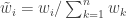
First generate a sample from and compute weights . Then compute normalised weights . Generate a new sample of size by sampling times with replacement from the original sample with the probability of choosing each value determined by its normalised weight.

As an example, consider using a sample from the Cauchy distribution as an auxiliary distribution for approximately sampling standard normal random quantities. We can do this using a few lines of R as follows.

n=1000
xa=rcauchy(n)
w=dnorm(xa)/dcauchy(xa)
x=sample(xa,n,prob=w,replace=TRUE)
hist(x,30)
mean(w)

Note that we don’t actually need to compute the normalised weights, as the sample function will do this for us. Note also that the average weight will be close to one. It should be clear that the expected value of the weights will be exactly 1 when both the target and auxiliary densities are correctly normalised. Also note that the procedure can be used when one or both of the densities are not correctly normalised, since the weights will be normalised prior to sampling anyway. Note that in this case the expected weight will be the (ratio of) normalising constant(s), and so looking at the average weight will give an estimate of the normalising constant.

Note that the importance sampling procedure is approximate. Unlike a technique such as rejection sampling, which leads to samples having exactly the correct distribution, this is not the case here. Indeed, it is clear that in the case, the final sample will be exactly drawn from the auxiliary and not the target. The procedure is asymptotic, in that it improves as the sample size increases, tending to the exact target as .

We can understand why importance resampling works by first considering the univariate case, using correctly normalised densities. Consider a very large number of particles, . The proportion of the auxiliary samples falling in a small interval will be , corresponding to roughly particles. The weight for each of those particles will be , and since the expected weight of a random particle is 1, the sum of all weights will be (roughly) , leading to normalised weights for the particles near of . The combined weight of all particles in is therefore . Clearly then, when we resample times we expect to select roughly particles from this interval. This corresponds to a proportion , corresponding to a density of in the final sample.

Obviously the above argument is very informal, but can be tightened up into a reasonably rigorous proof for the 1d case without too much effort, and the multivariate extension is also reasonably clear.

The bootstrap particle filter

The bootstrap particle filter is an iterative method for carrying out Bayesian inference for dynamic state space (partially observed Markov process) models, sometimes also known as hidden Markov models (HMMs). Here, an unobserved Markov process, governed by a transition kernel is partially observed via some measurement model leading to data . The idea is to make inference for the hidden states given the data . The method is a very simple application of the importance resampling technique. At each time, , we assume that we have a (approximate) sample from and use importance resampling to generate an approximate sample from .

More precisely, the procedure is initialised with a sample from with uniform normalised weights . Then suppose that we have a weighted sample from . First generate an equally weighted sample by resampling with replacement times to obtain (giving an approximate random sample from ). Note that each sample is independently drawn from . Next propagate each particle forward according to the Markov process model by sampling (giving an approximate random sample from ). Then for each of the new particles, compute a weight , and then a normalised weight .

It is clear from our understanding of importance resampling that these weights are appropriate for representing a sample from , and so the particles and weights can be propagated forward to the next time point. It is also clear that the average weight at each time gives an estimate of the marginal likelihood of the current data point given the data so far. So we define

and

Again, from our understanding of importance resampling, it should be reasonably clear that is a consistent estimator of . It is much less clear, but nevertheless true that this estimator is also unbiased. The standard reference for this fact is Del Moral (2004), but this is a rather technical monograph. A much more accessible proof (for a very general particle filter) is given in Pitt et al (2011).

It should therefore be clear that if one is interested in developing MCMC algorithms for state space models, one can use a pseudo-marginal MCMC scheme, substituting in from a bootstrap particle filter in place of . This turns out to be a simple special case of the particle marginal Metropolis-Hastings (PMMH) algorithm described in Andreiu et al (2010). However, the PMMH algorithm in fact has the full joint posterior as its target. I will explain the PMMH algorithm in a subsequent post.

The pseudo-marginal approach to “exact approximate” MCMC algorithms

Motivation and background

In this post I will try and explain an important idea behind some recent developments in MCMC theory. First, let me give some motivation. Suppose you are trying to implement a Metropolis-Hastings algorithm, as discussed in a previous post (required reading!), but a key likelihood term needed for the acceptance ratio is difficult to evaluate (most likely it is a marginal likelihood of some sort). If it is possible to obtain a Monte-Carlo estimate for that likelihood term (which it sometimes is, for example, using importance sampling), one could obviously just plug it in to the acceptance ratio and hope for the best. What is not at all obvious is that if your Monte-Carlo estimate satisfies some fairly weak property then the equilibrium distribution of the Markov chain will remain exactly as it would be if the exact likelihood had been available. Furthermore, it is exact even if the Monte-Carlo estimate is very noisy and imprecise (though the mixing of the chain will be poorer in this case). This is the “exact approximate” pseudo-marginal MCMC approach. To give credit where it is due, the idea was first introduced by Mark Beaumont in Beaumont (2003), where he was using an importance sampling based approximate likelihood in the context of a statistical genetics example. This was later picked up by Christophe Andrieu and Gareth Roberts, who studied the technical properties of the approach in Andrieu and Roberts (2009). The idea is turning out to be useful in several contexts, and in particular, underpins the interesting new Particle MCMC algorithms of Andrieu et al (2010), which I will discuss in a future post. I’ve heard Mark, Christophe, Gareth and probably others present this concept, but this post is most strongly inspired by a talk that Christophe gave at the IMS 2010 meeting in Gothenburg this summer.

The pseudo-marginal Metropolis-Hastings algorithm

Let’s focus on the simplest version of the problem, where we want to sample from a target using a proposal . As explained previously, the required Metropolis-Hastings acceptance ratio will take the form

Here we are assuming that is difficult to evaluate (usually because it is a marginalised version of some higher-dimensional distribution), but that a Monte-Carlo estimate of , which we shall denote , can be computed. We can obviously just substitute this estimate into the acceptance ratio to get

but it is not immediately clear that in many cases this will lead to the Markov chain having an equilibrium distribution that is exactly . It turns out that it is sufficient that the likelihood estimate, is non-negative, and unbiased, in the sense that , where the expectation is with respect to the Monte-Carlo error for a given fixed value of . In fact, as we shall see, this condition is actually a bit stronger than is really required.

Put , representing the noise in the Monte-Carlo estimate of , and suppose that (note that in an abuse of notation, the function is unrelated to ). The main condition we will assume is that , where is a constant independent of . In the case of , we have the (typical) special case of . For now, we will also assume that , but we will consider relaxing this constraint later.

The key to understanding the pseudo-marginal approach is to realise that at each iteration of the MCMC algorithm a new value of is being proposed in addition to a new value for . If we regard the proposal mechanism as a joint update of and , it is clear that the proposal generates from the density , and we can re-write our “approximate” acceptance ratio as

Inspection of this acceptance ratio reveals that the target of the chain must be (proportional to)

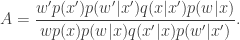
This is a joint density for , but the marginal for can be obtained by integrating over the range of with respect to . Using the fact that , this then clearly gives a density proportional to , and this is precisely the target that we require. Note that for this to work, we must keep the old value of from one iteration to the next – that is, we must keep and re-use our noisy value to include in the acceptance ratio for our next MCMC iteration – we should not compute a new Monte-Carlo estimate for the likelihood of the old state of the chain.

Examples

We will consider again the example from the previous post – simulation of a chain with a N(0,1) target using uniform innovations. Using R, the main MCMC loop takes the form

pmmcmc<-function(n=1000,alpha=0.5) 
{
        vec=vector("numeric", n)
        x=0
        oldlik=noisydnorm(x)
        vec[1]=x
        for (i in 2:n) {
                innov=runif(1,-alpha,alpha)
                can=x+innov
                lik=noisydnorm(can)
                aprob=lik/oldlik
                u=runif(1)
                if (u < aprob) { 
                        x=can
                        oldlik=lik
			}
                vec[i]=x
        }
        vec
}

Here we are assuming that we are unable to compute dnorm exactly, but instead only a Monte-Carlo estimate called noisydnorm. We can start with the following implementation

noisydnorm<-function(z)
{
	dnorm(z)*rexp(1,1)
}

Each time this function is called, it will return a non-negative random quantity whose expectation is dnorm(z). We can now run this code as follows.

plot.mcmc<-function(mcmc.out)
{
	op=par(mfrow=c(2,2))
	plot(ts(mcmc.out),col=2)
	hist(mcmc.out,30,col=3)
	qqnorm(mcmc.out,col=4)
	abline(0,1,col=2)
	acf(mcmc.out,col=2,lag.max=100)
	par(op)
}

metrop.out<-pmmcmc(10000,1)
plot.mcmc(metrop.out)

MCMC output and convergence diagnostics

So we see that we have exactly the right N(0,1) target, despite using the (very) noisy noisydnorm function in place of the dnorm function. This noisy likelihood function is clearly unbiased. However, as already discussed, a constant bias in the noise is also acceptable, as the following function shows.

noisydnorm<-function(z)
{
	dnorm(z)*rexp(1,2)
}

Re-running the code with this function also leads to the correct equilibrium distribution for the chain. However, it really does matter that the bias is independent of the state of the chain, as the following function shows.

noisydnorm<-function(z)
{
	dnorm(z)*rexp(1,0.1+10*z*z)
}

Running with this function leads to the wrong equilibrium. However, it is OK for the distribution of the noise to depend on the state, as long as its expectation does not. The following function illustrates this.

noisydnorm<-function(z)
{
	dnorm(z)*rgamma(1,0.1+10*z*z,0.1+10*z*z)
}

This works just fine. So far we have been assuming that our noisy likelihood estimates are non-negative. This is clearly desirable, as otherwise we could wind up with negative Metropolis-Hasting ratios. However, as long as we are careful about exactly what we mean, even this non-negativity condition may be relaxed. The following function illustrates the point.

noisydnorm<-function(z)
{
	dnorm(z)*rnorm(1,1)
}

Despite the fact that this function will often produce negative values, the equilibrium distribution of the chain still seems to be correct! An even more spectacular example follows.

noisydnorm<-function(z)
{
	dnorm(z)*rnorm(1,0)
}

Astonishingly, this one works too, despite having an expected value of zero! However, the following doesn’t work, even though it too has a constant expectation of zero.

noisydnorm<-function(z)
{
	dnorm(z)*rnorm(1,0,0.1+10*z*z)
}

I don’t have time to explain exactly what is going on here, so the precise details are left as an exercise for the reader. Suffice to say that the key requirement is that it is the distribution of W conditioned to be non-negative which must have the constant bias property – something clearly violated by the final noisydnorm example.

Before finishing this post, it is worth re-emphasising the issue of re-using old Monte-Carlo estimates. The following function will not work (exactly), though in the case of good Monte-Carlo estimates will often work tolerably well.

approxmcmc<-function(n=1000,alpha=0.5) 
{
        vec=vector("numeric", n)
        x=0
        vec[1]=x
        for (i in 2:n) {
                innov=runif(1,-alpha,alpha)
                can=x+innov
                lik=noisydnorm(can)
                oldlik=noisydnorm(x)
                aprob=lik/oldlik
                u=runif(1)
                if (u < aprob) { 
                        x=can
			}
                vec[i]=x
        }
        vec
}

In a subsequent post I will show how these ideas can be put into practice in the context of a Bayesian inference example.