Gibbs – Darren Wilkinson's blog

Bayesian inference for a logistic regression model (Part 6)

Part 6: Hamiltonian Monte Carlo (HMC)

Introduction

This is the sixth part in a series of posts on MCMC-based Bayesian inference for a logistic regression model. If you are new to this series, please go back to Part 1.

In the previous post we saw how to construct an MCMC algorithm utilising gradient information by considering a Langevin equation having our target distribution of interest as its equilibrium. This equation has a physical interpretation in terms of the stochastic dynamics of a particle in a potential equal to minus the log of the target density. It turns out that thinking about the deterministic dynamics of a particle in such a potential can lead to more efficient MCMC algorithms.

Hamiltonian dynamics

Hamiltonian dynamics is often presented as an extension of a fairly general version of Lagrangian dynamics. However, for our purposes a rather simple version is quite sufficient, based on basic concepts from Newtonian dynamics, familiar from school. Inspired by our Langevin example, we will consider the dynamics of a particle in a potential function $V(q)$ . We will see later why we want $V(q) = -\log \pi(q)$ for our target of interest, $\pi(\cdot)$ . In the context of Hamiltonian (and Lagrangian) dynamics we typically use $q$ as our position variable, rather than $x$ .

The potential function induces a (conservative) force on the particle equal to $-\nabla V(q)$ when the particle is at position $q$ . Then Newton’s second law of motion, "F=ma", takes the form

$\displaystyle \nabla V(q) + m \ddot{q} = 0.$

In Newtonian mechanics, we often consider the position vector $q$ as 3-dimensional. Here it will be $n$ -dimensional, where $n$ is the number of variables in our target. We can then think of our second law as governing a single $n$ -dimensional particle of mass $m$ , or $n$ one-dimensional particles all of mass $m$ . But in this latter case, there is no need to assume that all particles have the same mass, and we could instead write our law of motion as

$\displaystyle \nabla V(q) + M \ddot{q} = 0,$

where $M$ is a diagonal matrix. But in fact, since we could change coordinates, there’s no reason to require that $M$ is diagonal. All we need is that $M$ is positive definite, so that we don’t have negative mass in any coordinate direction.

We will take the above equation as the fundamental law governing our dynamical system of interest. The motivation from Newtonian dynamics is interesting, but not required. What is important is that the dynamics of such a system are conservative, in a way that we will shortly make precise.

Our law of motion is a second-order differential equation, since it involves the second derivative of $q$ wrt time. If you’ve ever studied differential equations, you’ll know that there is an easy way to turn a second order equation into a first order equation with twice the dimension by augmenting the system with the velocities. Here, it is more convenient to augment the system with "momentum" variables, $p$ , which we define as $p = M\dot{q}$ . Then we can write our second order system as a pair of first order equations

$\displaystyle \dot{q} = M^{-1}p$

$\displaystyle \dot{p} = -\nabla V(q)$

These are, in fact, Hamilton’s equations for this system, though this isn’t how they are typically written.

If we define the kinetic energy as

$\displaystyle T(p) = \frac{1}{2}p^\text{T}M^{-1}p,$

then the Hamiltonian

$\displaystyle H(q,p) = V(q) + T(p),$

representing the total energy in the system, is conserved, since

$\displaystyle \dot{H} = \nabla V\cdot \dot{q} + \dot{p}^\text{T}M^{-1}p = \nabla V\cdot \dot{q} + \dot{p}^\text{T}\dot{q} = [\nabla V + \dot{p}]\cdot\dot{q} = 0.$

So, if we obey our Hamiltonian dynamics, our trajectory in $(q,p)$ -space will follow contours of the Hamiltonian. It’s also clear that the system is time-reversible, so flipping the sign of the momentum $p$ and integrating will exactly reverse the direction in which the contours are traversed. Another quite important property of Hamiltonian dynamics is that they are volume preserving. This can be verified by checking that the divergence of the flow is zero.

$\displaystyle \nabla\cdot(\dot{q},\dot{p}) = \nabla_q\cdot\dot{q} + \nabla_p\cdot\dot{p} = 0,$

since $\dot{q}$ is a function of $p$ only and $\dot{p}$ is a function of $q$ only.

Hamiltonian Monte Carlo (HMC)

In Hamiltonian Monte Carlo we introduce an augmented target distribution,

$\displaystyle \tilde \pi(q,p) \propto \exp[-H(q,p)]$

It is clear from this definition that moves leaving the Hamiltonian invariant will also leave the augmented target density unchanged. By following the Hamiltonian dynamics, we will be able to make big (reversible) moves in the space that will be accepted with high probability. Also, our target factorises into two independent components as

$\displaystyle \tilde \pi(q,p) \propto \exp[-V(q)]\exp[-T(p)],$

and so choosing $V(q)=-\log \pi(q)$ will ensure that the $q$ -marginal is our real target of interest, $\pi(\cdot)$ . It’s also clear that our $p$ -marginal is $\mathcal N(0,M)$ . This is also the full-conditional for $p$ , so re-sampling $p$ from this distribution and leaving $q$ unchanged is a Gibbs move that will leave the augmented target invariant. Re-sampling $p$ will be necessary to properly explore our augmented target, since this will move us to a different contour of $H$ .

So, an idealised version of HMC would proceed as follows: First, update $p$ by sampling from its known tractable marginal. Second, update $p$ and $q$ jointly by following the Hamiltonian dynamics. If this second move is regarded as a (deterministic) reversible M-H proposal, it will be accepted with probability one since it leaves the augmented target density unchanged. If we could exactly integrate Hamilton’s equations, this would be fine. But in practice, we will need to use some imperfect numerical method for the integration step. But just as for MALA, we can regard the numerical method as a M-H proposal and correct for the fact that it is imperfect, preserving the exact augmented target distribution.

Hamiltonian systems admit nice numerical integration schemes called symplectic integrators. In HMC a simple alternating Euler method is typically used, known as the leap-frog algorithm. The component updates are all shear transformations, and therefore volume preserving, and exact reversibility is ensured by starting and ending with a half-step update of the momentum variables. In principle, to ensure reversibility of the proposal the momentum variables should be sign-flipped (reversed) to finish, but in practice this doesn’t matter since it doesn’t affect the evaluation of the Hamiltonian and it will then get refreshed, anyway.

So, advancing our system by a time step $\epsilon$ can be done with

$\displaystyle p(t+\epsilon/2) := p(t) - \frac{\epsilon}{2}\nabla V(q(t))$

$\displaystyle q(t+\epsilon) := q(t) + \epsilon M^{-1}p(t+\epsilon/2)$

$\displaystyle p(t+\epsilon) := p(t+\epsilon/2) - \frac{\epsilon}{2}\nabla V(q(t+\epsilon))$

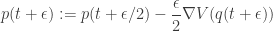
It is clear that if many such updates are chained together, adjacent momentum updates can be collapsed together, giving rise to the "leap-frog" nature of the algorithm, and therefore requiring roughly one gradient evaluation per $\epsilon$ update, rather than two. Since this integrator is volume preserving and exactly reversible, for reasonably small $\epsilon$ it follows the Hamiltonian dynamics reasonably well, but not exactly, and so it does not exactly preserve the Hamiltonian. However, it does make a good M-H proposal, and reasonable acceptance probabilities can often be obtained by chaining together $l$ updates to advance the time of the system by $T=l\epsilon$ . The "optimal" value of $l$ and $\epsilon$ will be highly problem dependent, but values of $l=20$ or $l=50$ are not unusual. There are various more-or-less standard methods for tuning these, but we will not consider them here.

Note that since our HMC update on the augmented space consists of a Gibbs move and a M-H update, it is important that our M-H kernel does not keep or thread through the old log target density from the previous M-H update, since the Gibbs move will have changed it in the meantime.

Implementations

R

We need a M-H kernel that does not thread through the old log density.

mhKernel = function(logPost, rprop)
    function(x) {
        prop = rprop(x)
        a = logPost(prop) - logPost(x)
        if (log(runif(1)) < a)
            prop
        else
            x
    }

We can then use this to construct a M-H move as part of our HMC update.

hmcKernel = function(lpi, glpi, eps = 1e-4, l=10, dmm = 1) {
    sdmm = sqrt(dmm)
    leapf = function(q, p) {
        p = p + 0.5*eps*glpi(q)
        for (i in 1:l) {
            q = q + eps*p/dmm
            if (i < l)
                p = p + eps*glpi(q)
            else
                p = p + 0.5*eps*glpi(q)
        }
        list(q=q, p=-p)
    }
    alpi = function(x)
        lpi(x$q) - 0.5*sum((x$p^2)/dmm)
    rprop = function(x)
        leapf(x$q, x$p)
    mhk = mhKernel(alpi, rprop)
    function(q) {
        d = length(q)
        x = list(q=q, p=rnorm(d, 0, sdmm))
        mhk(x)$q
    }
}

See the full runnable script for further details.

Python

First a M-H kernel,

def mhKernel(lpost, rprop):
    def kernel(x):
        prop = rprop(x)
        a = lpost(prop) - lpost(x)
        if (np.log(np.random.rand()) < a):
            x = prop
        return x
    return kernel

and then an HMC kernel.

def hmcKernel(lpi, glpi, eps = 1e-4, l=10, dmm = 1):
    sdmm = np.sqrt(dmm)
    def leapf(q, p):    
        p = p + 0.5*eps*glpi(q)
        for i in range(l):
            q = q + eps*p/dmm
            if (i < l-1):
                p = p + eps*glpi(q)
            else:
                p = p + 0.5*eps*glpi(q)
        return (q, -p)
    def alpi(x):
        (q, p) = x
        return lpi(q) - 0.5*np.sum((p**2)/dmm)
    def rprop(x):
        (q, p) = x
        return leapf(q, p)
    mhk = mhKernel(alpi, rprop)
    def kern(q):
        d = len(q)
        p = np.random.randn(d)*sdmm
        return mhk((q, p))[0]
    return kern

See the full runnable script for further details.

JAX

Again, we want an appropriate M-H kernel,

def mhKernel(lpost, rprop, dprop = jit(lambda new, old: 1.)):
    @jit
    def kernel(key, x):
        key0, key1 = jax.random.split(key)
        prop = rprop(key0, x)
        ll = lpost(x)
        lp = lpost(prop)
        a = lp - ll + dprop(x, prop) - dprop(prop, x)
        accept = (jnp.log(jax.random.uniform(key1)) < a)
        return jnp.where(accept, prop, x)
    return kernel

and then an HMC kernel.

def hmcKernel(lpi, glpi, eps = 1e-4, l = 10, dmm = 1):
    sdmm = jnp.sqrt(dmm)
    @jit
    def leapf(q, p):    
        p = p + 0.5*eps*glpi(q)
        for i in range(l):
            q = q + eps*p/dmm
            if (i < l-1):
                p = p + eps*glpi(q)
            else:
                p = p + 0.5*eps*glpi(q)
        return jnp.concatenate((q, -p))
    @jit
    def alpi(x):
        d = len(x) // 2
        return lpi(x[jnp.array(range(d))]) - 0.5*jnp.sum((x[jnp.array(range(d,2*d))]**2)/dmm)
    @jit
    def rprop(k, x):
        d = len(x) // 2
        return leapf(x[jnp.array(range(d))], x[jnp.array(range(d, 2*d))])
    mhk = mhKernel(alpi, rprop)
    @jit
    def kern(k, q):
        key0, key1 = jax.random.split(k)
        d = len(q)
        x = jnp.concatenate((q, jax.random.normal(key0, [d])*sdmm))
        return mhk(key1, x)[jnp.array(range(d))]
    return kern

There is something a little bit strange about this implementation, since the proposal for the M-H move is deterministic, the function rprop just ignores the RNG key that is passed to it. We could tidy this up by making a M-H function especially for deterministic proposals. We won’t pursue this here, but this issue will crop up again later in some of the other functional languages.

See the full runnable script for further details.

Scala

A M-H kernel,

def mhKern[S](
    logPost: S => Double, rprop: S => S,
    dprop: (S, S) => Double = (n: S, o: S) => 1.0
  ): (S) => S =
    val r = Uniform(0.0,1.0)
    x0 =>
      val x = rprop(x0)
      val ll0 = logPost(x0)
      val ll = logPost(x)
      val a = ll - ll0 + dprop(x0, x) - dprop(x, x0)
      if (math.log(r.draw()) < a) x else x0

and a HMC kernel.

def hmcKernel(lpi: DVD => Double, glpi: DVD => DVD, dmm: DVD,
  eps: Double = 1e-4, l: Int = 10) =
  val sdmm = sqrt(dmm)
  def leapf(q: DVD, p: DVD): (DVD, DVD) = 
    @tailrec def go(q0: DVD, p0: DVD, l: Int): (DVD, DVD) =
      val q = q0 + eps*(p0/:/dmm)
      val p = if (l > 1)
        p0 + eps*glpi(q)
      else
        p0 + 0.5*eps*glpi(q)
      if (l == 1)
        (q, -p)
      else
        go(q, p, l-1)
    go(q, p + 0.5*eps*glpi(q), l)
  def alpi(x: (DVD, DVD)): Double =
    val (q, p) = x
    lpi(q) - 0.5*sum(pow(p,2) /:/ dmm)
  def rprop(x: (DVD, DVD)): (DVD, DVD) =
    val (q, p) = x
    leapf(q, p)
  val mhk = mhKern(alpi, rprop)
  (q: DVD) =>
    val d = q.length
    val p = sdmm map (sd => Gaussian(0,sd).draw())
    mhk((q, p))._1

See the full runnable script for further details.

Haskell

A M-H kernel:

mdKernel :: (StatefulGen g m) => (s -> Double) -> (s -> s) -> g -> s -> m s
mdKernel logPost prop g x0 = do
  let x = prop x0
  let ll0 = logPost x0
  let ll = logPost x
  let a = ll - ll0
  u <- (genContVar (uniformDistr 0.0 1.0)) g
  let next = if ((log u) < a)
        then x
        else x0
  return next

Note that here we are using a M-H kernel specifically for deterministic proposals, since there is no non-determinism signalled in the type signature of prop. We can then use this to construct our HMC kernel.

hmcKernel :: (StatefulGen g m) =>
  (Vector Double -> Double) -> (Vector Double -> Vector Double) -> Vector Double ->
  Double -> Int -> g ->
  Vector Double -> m (Vector Double)
hmcKernel lpi glpi dmm eps l g = let
  sdmm = cmap sqrt dmm
  leapf q p = let
    go q0 p0 l = let
      q = q0 + (scalar eps)*p0/dmm
      p = if (l > 1)
        then p0 + (scalar eps)*(glpi q)
        else p0 + (scalar (eps/2))*(glpi q)
      in if (l == 1)
      then (q, -p)
      else go q p (l - 1)
    in go q (p + (scalar (eps/2))*(glpi q)) l
  alpi x = let
    (q, p) = x
    in (lpi q) - 0.5*(sumElements (p*p/dmm))
  prop x = let
    (q, p) = x
    in leapf q p
  mk = mdKernel alpi prop g
  in (\q0 -> do
         let d = size q0
         zl <- (replicateM d . genContVar (normalDistr 0.0 1.0)) g
         let z = fromList zl
         let p0 = sdmm * z
         (q, p) <- mk (q0, p0)
         return q)

See the full runnable script for further details.

Dex

Again we can use a M-H kernel specific to deterministic proposals.

def mdKernel {s} (lpost: s -> Float) (prop: s -> s)
    (x0: s) (k: Key) : s =
  x = prop x0
  ll0 = lpost x0
  ll = lpost x
  a = ll - ll0
  u = rand k
  select (log u < a) x x0

and use this to construct an HMC kernel.

def hmcKernel {n} (lpi: (Fin n)=>Float -> Float)
    (dmm: (Fin n)=>Float) (eps: Float) (l: Nat)
    (q0: (Fin n)=>Float) (k: Key) : (Fin n)=>Float =
  sdmm = sqrt dmm
  idmm = map (\x. 1.0/x) dmm
  glpi = grad lpi
  def leapf (q0: (Fin n)=>Float) (p0: (Fin n)=>Float) :
      ((Fin n)=>Float & (Fin n)=>Float) =
    p1 = p0 + (eps/2) .* (glpi q0)
    q1 = q0 + eps .* (p1*idmm)
    (q, p) = apply_n l (q1, p1) \(qo, po).
      pn = po + eps .* (glpi qo)
      qn = qo + eps .* (pn*idmm)
      (qn, pn)
    pf = p + (eps/2) .* (glpi q)
    (q, -pf)
  def alpi (qp: ((Fin n)=>Float & (Fin n)=>Float)) : Float =
    (q, p) = qp
    (lpi q) - 0.5*(sum (p*p*idmm))
  def prop (qp: ((Fin n)=>Float & (Fin n)=>Float)) :
      ((Fin n)=>Float & (Fin n)=>Float) =
    (q, p) = qp
    leapf q p
  mk = mdKernel alpi prop
  [k1, k2] = split_key k
  z = randn_vec k1
  p0 = sdmm * z
  (q, p) = mk (q0, p0) k2
  q

Note that the gradient is obtained via automatic differentiation. See the full runnable script for details.

Next steps

This was the main place that I was trying to get to when I started this series of posts. For differentiable log-posteriors (as we have in the case of Bayesian logistic regression), HMC is a pretty good algorithm for reasonably efficient posterior exploration. But there are lots of places we could go from here. We could explore the tuning of MCMC algorithms, or HMC extensions such as NUTS. We could look at MCMC algorithms that are specifically tailored to the logistic regression problem, or we could look at new MCMC algorithms for differentiable targets based on piecewise deterministic Markov processes. Alternatively, we could temporarily abandon MCMC and look at SMC or ABC approaches. Another possibility would be to abandon this multi-language approach and have a bit of a deep dive into Dex, which I think has the potential to be a great programming language for statistical computing. All of these are possibilities for the future, but I’ve a busy few weeks coming up, so the frequency of these posts is likely to substantially decrease.

Remember that all of the code associated with this series of posts is available from this github repo.

Comonads for scientific and statistical computing in Scala

Introduction

In a previous post I’ve given a brief introduction to monads in Scala, aimed at people interested in scientific and statistical computing. Monads are a concept from category theory which turn out to be exceptionally useful for solving many problems in functional programming. But most categorical concepts have a dual, usually prefixed with “co”, so the dual of a monad is the comonad. Comonads turn out to be especially useful for formulating algorithms from scientific and statistical computing in an elegant way. In this post I’ll illustrate their use in signal processing, image processing, numerical integration of PDEs, and Gibbs sampling (of an Ising model). Comonads enable the extension of a local computation to a global computation, and this pattern crops up all over the place in statistical computing.

Monads and comonads

Simplifying massively, from the viewpoint of a Scala programmer, a monad is a mappable (functor) type class augmented with the methods pure and flatMap:

trait Monad[M[_]] extends Functor[M] {
  def pure[T](v: T): M[T]
  def flatMap[T,S](v: M[T])(f: T => M[S]): M[S]
}

In category theory, the dual of a concept is typically obtained by “reversing the arrows”. Here that means reversing the direction of the methods pure and flatMap to get extract and coflatMap, respectively.

trait Comonad[W[_]] extends Functor[W] {
  def extract[T](v: W[T]): T
  def coflatMap[T,S](v: W[T])(f: W[T] => S): W[S]
}

So, while pure allows you to wrap plain values in a monad, extract allows you to get a value out of a comonad. So you can always get a value out of a comonad (unlike a monad). Similarly, while flatMap allows you to transform a monad using a function returning a monad, coflatMap allows you to transform a comonad using a function which collapses a comonad to a single value. It is coflatMap (sometimes called extend) which can extend a local computation (producing a single value) to the entire comonad. We’ll look at how that works in the context of some familiar examples.

Applying a linear filter to a data stream

One of the simplest examples of a comonad is an infinite stream of data. I’ve discussed streams in a previous post. By focusing on infinite streams we know the stream will never be empty, so there will always be a value that we can extract. Which value does extract give? For a Stream encoded as some kind of lazy list, the only value we actually know is the value at the head of the stream, with subsequent values to be lazily computed as required. So the head of the list is the only reasonable value for extract to return.

Understanding coflatMap is a bit more tricky, but it is coflatMap that provides us with the power to apply a non-trivial statistical computation to the stream. The input is a function which transforms a stream into a value. In our example, that will be a function which computes a weighted average of the first few values and returns that weighted average as the result. But the return type of coflatMap must be a stream of such computations. Following the types, a few minutes thought reveals that the only reasonable thing to do is to return the stream formed by applying the weighted average function to all sub-streams, recursively. So, for a Stream s (of type Stream[T]) and an input function f: W[T] => S, we form a stream whose head is f(s) and whose tail is coflatMap(f) applied to s.tail. Again, since we are working with an infinite stream, we don’t have to worry about whether or not the tail is empty. This gives us our comonadic Stream, and it is exactly what we need for applying a linear filter to the data stream.

In Scala, Cats is a library providing type classes from Category theory, and instances of those type classes for parametrised types in the standard library. In particular, it provides us with comonadic functionality for the standard Scala Stream. Let’s start by defining a stream corresponding to the logistic map.

import cats._
import cats.implicits._

val lam = 3.7
def s = Stream.iterate(0.5)(x => lam*x*(1-x))
s.take(10).toList
// res0: List[Double] = List(0.5, 0.925, 0.25668749999999985,
//  0.7059564011718747, 0.7680532550204203, 0.6591455741499428, ...

Let us now suppose that we want to apply a linear filter to this stream, in order to smooth the values. The idea behind using comonads is that you figure out how to generate one desired value, and let coflatMap take care of applying the same logic to the rest of the structure. So here, we need a function to generate the first filtered value (since extract is focused on the head of the stream). A simple first attempt a function to do this might look like the following.

  def linearFilterS(weights: Stream[Double])(s: Stream[Double]): Double =
    (weights, s).parMapN(_*_).sum

This aligns each weight in parallel with a corresponding value from the stream, and combines them using multiplication. The resulting (hopefully finite length) stream is then summed (with addition). We can test this with

linearFilterS(Stream(0.25,0.5,0.25))(s)
// res1: Double = 0.651671875

and let coflatMap extend this computation to the rest of the stream with something like:

s.coflatMap(linearFilterS(Stream(0.25,0.5,0.25))).take(5).toList
// res2: List[Double] = List(0.651671875, 0.5360828502929686, ...

This is all completely fine, but our linearFilterS function is specific to the Stream comonad, despite the fact that all we’ve used about it in the function is that it is a parallelly composable and foldable. We can make this much more generic as follows:

  def linearFilter[F[_]: Foldable, G[_]](
    weights: F[Double], s: F[Double]
  )(implicit ev: NonEmptyParallel[F, G]): Double =
    (weights, s).parMapN(_*_).fold

This uses some fairly advanced Scala concepts which I don’t want to get into right now (I should also acknowledge that I had trouble getting the syntax right for this, and got help from Fabio Labella (@SystemFw) on the Cats gitter channel). But this version is more generic, and can be used to linearly filter other data structures than Stream. We can use this for regular Streams as follows:

s.coflatMap(s => linearFilter(Stream(0.25,0.5,0.25),s))
// res3: scala.collection.immutable.Stream[Double] = Stream(0.651671875, ?)

But we can apply this new filter to other collections. This could be other, more sophisticated, streams such as provided by FS2, Monix or Akka streams. But it could also be a non-stream collection, such as List:

val sl = s.take(10).toList
sl.coflatMap(sl => linearFilter(List(0.25,0.5,0.25),sl))
// res4: List[Double] = List(0.651671875, 0.5360828502929686, ...

Assuming that we have the Breeze scientific library available, we can plot the raw and smoothed trajectories.

def myFilter(s: Stream[Double]): Double =
  linearFilter(Stream(0.25, 0.5, 0.25),s)
val n = 500
import breeze.plot._
import breeze.linalg._
val fig = Figure(s"The (smoothed) logistic map (lambda=$lam)")
val p0 = fig.subplot(3,1,0)
p0 += plot(linspace(1,n,n),s.take(n))
p0.ylim = (0.0,1.0)
p0.title = s"The logistic map (lambda=$lam)"
val p1 = fig.subplot(3,1,1)
p1 += plot(linspace(1,n,n),s.coflatMap(myFilter).take(n))
p1.ylim = (0.0,1.0)
p1.title = "Smoothed by a simple linear filter"
val p2 = fig.subplot(3,1,2)
p2 += plot(linspace(1,n,n),s.coflatMap(myFilter).coflatMap(myFilter).coflatMap(myFilter).coflatMap(myFilter).coflatMap(myFilter).take(n))
p2.ylim = (0.0,1.0)
p2.title = "Smoothed with 5 applications of the linear filter"
fig.refresh

Image processing and the heat equation

Streaming data is in no way the only context in which a comonadic approach facilitates an elegant approach to scientific and statistical computing. Comonads crop up anywhere where we want to extend a computation that is local to a small part of a data structure to the full data structure. Another commonly cited area of application of comonadic approaches is image processing (I should acknowledge that this section of the post is very much influenced by a blog post on comonadic image processing in Haskell). However, the kinds of operations used in image processing are in many cases very similar to the operations used in finite difference approaches to numerical integration of partial differential equations (PDEs) such as the heat equation, so in this section I will blur (sic) the distinction between the two, and numerically integrate the 2D heat equation in order to Gaussian blur a noisy image.

First we need a simple image type which can have pixels of arbitrary type T (this is very important – all functors must be fully type polymorphic).

  import scala.collection.parallel.immutable.ParVector
  case class Image[T](w: Int, h: Int, data: ParVector[T]) {
    def apply(x: Int, y: Int): T = data(x*h+y)
    def map[S](f: T => S): Image[S] = Image(w, h, data map f)
    def updated(x: Int, y: Int, value: T): Image[T] =
      Image(w,h,data.updated(x*h+y,value))
  }

Here I’ve chosen to back the image with a parallel immutable vector. This wasn’t necessary, but since this type has a map operation which automatically parallelises over multiple cores, any map operations applied to the image will be automatically parallelised. This will ultimately lead to all of our statistical computations being automatically parallelised without us having to think about it.

As it stands, this image isn’t comonadic, since it doesn’t implement extract or coflatMap. Unlike the case of Stream, there isn’t really a uniquely privileged pixel, so it’s not clear what extract should return. For many data structures of this type, we make them comonadic by adding a “cursor” pointing to a “current” element of interest, and use this as the focus for computations applied with coflatMap. This is simplest to explain by example. We can define our “pointed” image type as follows:

  case class PImage[T](x: Int, y: Int, image: Image[T]) {
    def extract: T = image(x, y)
    def map[S](f: T => S): PImage[S] = PImage(x, y, image map f)
    def coflatMap[S](f: PImage[T] => S): PImage[S] = PImage(
      x, y, Image(image.w, image.h,
      (0 until (image.w * image.h)).toVector.par.map(i => {
        val xx = i / image.h
        val yy = i % image.h
        f(PImage(xx, yy, image))
      })))

There is missing a closing brace, as I’m not quite finished. Here x and y represent the location of our cursor, so extract returns the value of the pixel indexed by our cursor. Similarly, coflatMap forms an image where the value of the image at each location is the result of applying the function f to the image which had the cursor set to that location. Clearly f should use the cursor in some way, otherwise the image will have the same value at every pixel location. Note that map and coflatMap operations will be automatically parallelised. The intuitive idea behind coflatMap is that it extends local computations. For the stream example, the local computation was a linear combination of nearby values. Similarly, in image analysis problems, we often want to apply a linear filter to nearby pixels. We can get at the pixel at the cursor location using extract, but we probably also want to be able to move the cursor around to nearby locations. We can do that by adding some appropriate methods to complete the class definition.

    def up: PImage[T] = {
      val py = y-1
      val ny = if (py >= 0) py else (py + image.h)
      PImage(x,ny,image)
    }
    def down: PImage[T] = {
      val py = y+1
      val ny = if (py < image.h) py else (py - image.h)
      PImage(x,ny,image)
    }
    def left: PImage[T] = {
      val px = x-1
      val nx = if (px >= 0) px else (px + image.w)
      PImage(nx,y,image)
    }
    def right: PImage[T] = {
      val px = x+1
      val nx = if (px < image.w) px else (px - image.w)
      PImage(nx,y,image)
    }
  }

Here each method returns a new pointed image with the cursor shifted by one pixel in the appropriate direction. Note that I’ve used periodic boundary conditions here, which often makes sense for numerical integration of PDEs, but makes less sense for real image analysis problems. Note that we have embedded all “indexing” issues inside the definition of our classes. Now that we have it, none of the statistical algorithms that we develop will involve any explicit indexing. This makes it much less likely to develop algorithms containing bugs corresponding to “off-by-one” or flipped axis errors.

This class is now fine for our requirements. But if we wanted Cats to understand that this structure is really a comonad (perhaps because we wanted to use derived methods, such as coflatten), we would need to provide evidence for this. The details aren’t especially important for this post, but we can do it simply as follows:

  implicit val pimageComonad = new Comonad[PImage] {
    def extract[A](wa: PImage[A]) = wa.extract
    def coflatMap[A,B](wa: PImage[A])(f: PImage[A] => B): PImage[B] =
      wa.coflatMap(f)
    def map[A,B](wa: PImage[A])(f: A => B): PImage[B] = wa.map(f)
  }

It’s handy to have some functions for converting Breeze dense matrices back and forth with our image class.

  import breeze.linalg.{Vector => BVec, _}
  def BDM2I[T](m: DenseMatrix[T]): Image[T] =
    Image(m.cols, m.rows, m.data.toVector.par)
  def I2BDM(im: Image[Double]): DenseMatrix[Double] =
    new DenseMatrix(im.h,im.w,im.data.toArray)

Now we are ready to see how to use this in practice. Let’s start by defining a very simple linear filter.

def fil(pi: PImage[Double]): Double = (2*pi.extract+
  pi.up.extract+pi.down.extract+pi.left.extract+pi.right.extract)/6.0

This simple filter can be used to “smooth” or “blur” an image. However, from a more sophisticated viewpoint, exactly this type of filter can be used to represent one time step of a numerical method for time integration of the 2D heat equation. Now we can simulate a noisy image and apply our filter to it using coflatMap:

import breeze.stats.distributions.Gaussian
val bdm = DenseMatrix.tabulate(200,250){case (i,j) => math.cos(
  0.1*math.sqrt((i*i+j*j))) + Gaussian(0.0,2.0).draw}
val pim0 = PImage(0,0,BDM2I(bdm))
def pims = Stream.iterate(pim0)(_.coflatMap(fil))

Note that here, rather than just applying the filter once, I’ve generated an infinite stream of pointed images, each one representing an additional application of the linear filter. Thus the sequence represents the time solution of the heat equation with initial condition corresponding to our simulated noisy image.

We can render the first few frames to check that it seems to be working.

import breeze.plot._
val fig = Figure("Diffusing a noisy image")
pims.take(25).zipWithIndex.foreach{case (pim,i) => {
  val p = fig.subplot(5,5,i)
  p += image(I2BDM(pim.image))
}}

Note that the numerical integration is carried out in parallel on all available cores automatically. Other image filters can be applied, and other (parabolic) PDEs can be numerically integrated in an essentially similar way.

Gibbs sampling the Ising model

Another place where the concept of extending a local computation to a global computation crops up is in the context of Gibbs sampling a high-dimensional probability distribution by cycling through the sampling of each variable in turn from its full-conditional distribution. I’ll illustrate this here using the Ising model, so that I can reuse the pointed image class from above, but the principles apply to any Gibbs sampling problem. In particular, the Ising model that we consider has a conditional independence structure corresponding to a graph of a square lattice. As above, we will use the comonadic structure of the square lattice to construct a Gibbs sampler. However, we can construct a Gibbs sampler for arbitrary graphical models in an essentially identical way by using a graph comonad.

Let’s begin by simulating a random image containing +/-1s:

import breeze.stats.distributions.{Binomial,Bernoulli}
val beta = 0.4
val bdm = DenseMatrix.tabulate(500,600){
  case (i,j) => (new Binomial(1,0.2)).draw
}.map(_*2 - 1) // random matrix of +/-1s
val pim0 = PImage(0,0,BDM2I(bdm))

We can use this to initialise our Gibbs sampler. We now need a Gibbs kernel representing the update of each pixel.

def gibbsKernel(pi: PImage[Int]): Int = {
   val sum = pi.up.extract+pi.down.extract+pi.left.extract+pi.right.extract
   val p1 = math.exp(beta*sum)
   val p2 = math.exp(-beta*sum)
   val probplus = p1/(p1+p2)
   if (new Bernoulli(probplus).draw) 1 else -1
}

So far so good, but there a couple of issues that we need to consider before we plough ahead and start coflatMapping. The first is that pure functional programmers will object to the fact that this function is not pure. It is a stochastic function which has the side-effect of mutating the random number state. I’m just going to duck that issue here, as I’ve previously discussed how to fix it using probability monads, and I don’t want it to distract us here.

However, there is a more fundamental problem here relating to parallel versus sequential application of Gibbs kernels. coflatMap is conceptually parallel (irrespective of how it is implemented) in that all computations used to build the new comonad are based solely on the information available in the starting comonad. OTOH, detailed balance of the Markov chain will only be preserved if the kernels for each pixel are applied sequentially. So if we coflatMap this kernel over the image we will break detailed balance. I should emphasise that this has nothing to do with the fact that I’ve implemented the pointed image using a parallel vector. Exactly the same issue would arise if we switched to backing the image with a regular (sequential) immutable Vector.

The trick here is to recognise that if we coloured alternate pixels black and white using a chequerboard pattern, then all of the black pixels are conditionally independent given the white pixels and vice-versa. Conditionally independent pixels can be updated by parallel application of a Gibbs kernel. So we just need separate kernels for updating odd and even pixels.

def oddKernel(pi: PImage[Int]): Int =
  if ((pi.x+pi.y) % 2 != 0) pi.extract else gibbsKernel(pi)
def evenKernel(pi: PImage[Int]): Int =
  if ((pi.x+pi.y) % 2 == 0) pi.extract else gibbsKernel(pi)

Each of these kernels can be coflatMapped over the image preserving detailed balance of the chain. So we can now construct an infinite stream of MCMC iterations as follows.

def pims = Stream.iterate(pim0)(_.coflatMap(oddKernel).
  coflatMap(evenKernel))

We can animate the first few iterations with:

import breeze.plot._
val fig = Figure("Ising model Gibbs sampler")
fig.width = 1000
fig.height = 800
pims.take(50).zipWithIndex.foreach{case (pim,i) => {
  print(s"$i ")
  fig.clear
  val p = fig.subplot(1,1,0)
  p.title = s"Ising model: frame $i"
  p += image(I2BDM(pim.image.map{_.toDouble}))
  fig.refresh
}}
println

Here I have a movie showing the first 1000 iterations. Note that youtube seems to have over-compressed it, but you should get the basic idea.

Again, note that this MCMC sampler runs in parallel on all available cores, automatically. This issue of odd/even pixel updating emphasises another issue that crops up a lot in functional programming: very often, thinking about how to express an algorithm functionally leads to an algorithm which parallelises naturally. For general graphs, figuring out which groups of nodes can be updated in parallel is essentially the graph colouring problem. I’ve discussed this previously in relation to parallel MCMC in:

Wilkinson, D. J. (2005) Parallel Bayesian Computation, Chapter 16 in E. J. Kontoghiorghes (ed.) Handbook of Parallel Computing and Statistics, Marcel Dekker/CRC Press, 481-512.

Calling Scala code from R using rscala

Introduction

In a previous post I looked at how to call Scala code from R using a CRAN package called jvmr. This package now seems to have been replaced by a new package called rscala. Like the old package, it requires a pre-existing Java installation. Unlike the old package, however, it no longer depends on rJava, which may simplify some installations. The rscala package is well documented, with a reference manual and a draft paper. In this post I will concentrate on the issue of calling sbt-based projects with dependencies on external libraries (such as breeze).

On a system with Java installed, it should be possible to install the rscala package with a simple

install.packages("rscala")

from the R command prompt. Calling

library(rscala)

will check that it has worked. The package will do a sensible search for a Scala installation and use it if it can find one. If it can’t find one (or can only find an installation older than 2.10.x), it will fail. In this case you can download and install a Scala installation specifically for rscala using the command

rscala::scalaInstall()

This option is likely to be attractive to sbt (or IDE) users who don’t like to rely on a system-wide scala installation.

A Gibbs sampler in Scala using Breeze

For illustration I’m going to use a Scala implementation of a Gibbs sampler. The Scala code, gibbs.scala is given below:

package gibbs

object Gibbs {

    import scala.annotation.tailrec
    import scala.math.sqrt
    import breeze.stats.distributions.{Gamma,Gaussian}

    case class State(x: Double, y: Double) {
      override def toString: String = x.toString + " , " + y + "\n"
    }

    def nextIter(s: State): State = {
      val newX = Gamma(3.0, 1.0/((s.y)*(s.y)+4.0)).draw
      State(newX, Gaussian(1.0/(newX+1), 1.0/sqrt(2*newX+2)).draw)
    }

    @tailrec def nextThinnedIter(s: State,left: Int): State =
      if (left==0) s else nextThinnedIter(nextIter(s),left-1)

    def genIters(s: State, stop: Int, thin: Int): List[State] = {
      @tailrec def go(s: State, left: Int, acc: List[State]): List[State] =
        if (left>0)
          go(nextThinnedIter(s,thin), left-1, s::acc)
          else acc
      go(s,stop,Nil).reverse
    }

    def main(args: Array[String]) = {
      if (args.length != 3) {
        println("Usage: sbt \"run <outFile> <iters> <thin>\"")
        sys.exit(1)
      } else {
        val outF=args(0)
        val iters=args(1).toInt
        val thin=args(2).toInt
        val out = genIters(State(0.0,0.0),iters,thin)
        val s = new java.io.FileWriter(outF)
        s.write("x , y\n")
        out map { it => s.write(it.toString) }
        s.close
      }
    }

}

This code requires Scala and the Breeze scientific library in order to build. We can specify this in a sbt build file, which should be called build.sbt and placed in the same directory as the Scala code.

name := "gibbs"

version := "0.1"

scalacOptions ++= Seq("-unchecked", "-deprecation", "-feature")

libraryDependencies  ++= Seq(
            "org.scalanlp" %% "breeze" % "0.10",
            "org.scalanlp" %% "breeze-natives" % "0.10"
)

resolvers ++= Seq(
            "Sonatype Snapshots" at "https://oss.sonatype.org/content/repositories/snapshots/",
            "Sonatype Releases" at "https://oss.sonatype.org/content/repositories/releases/"
)

scalaVersion := "2.11.6"

Now, from a system command prompt in the directory where the files are situated, it should be possible to download all dependencies and compile and run the code with a simple

sbt "run output.csv 50000 1000"

sbt magically manages all of the dependencies for us so that we don’t have to worry about them. However, for calling from R, it may be desirable to run the code without running sbt. There are several ways to achieve this, but the simplest is to build an “assembly jar” or “fat jar”, which is a Java byte-code file containing all code and libraries required in order to run the code on any system with a Java installation.

To build an assembly jar first create a subdirectory called project (the name matters), an in it place two files. The first should be called assembly.sbt, and should contain the line

addSbtPlugin("com.eed3si9n" % "sbt-assembly" % "0.13.0")

Since the version of the assembly tool can depend on the version of sbt, it is also best to fix the version of sbt being used by creating another file in the project directory called build.properties, which should contain the line

sbt.version=0.13.7

Now return to the parent directory and run

sbt assembly

If this works, it should create a fat jar target/scala-2.11/gibbs-assembly-0.1.jar. You can check it works by running

java -jar target/scala-2.11/gibbs-assembly-0.1.jar output.csv 10000 10

Assuming that it does, you are now ready to try running the code from within R.

Calling via R system calls

Since this code takes a relatively long time to run, calling it from R via simple system calls isn’t a particularly terrible idea. For example, we can do this from the R command prompt with the following commands

system("java -jar target/scala-2.11/gibbs-assembly-0.1.jar output.csv 50000 1000")
out=read.csv("output.csv")
library(smfsb)
mcmcSummary(out,rows=2)

This works fine, but is a bit clunky. Tighter integration between R and Scala would be useful, which is where rscala comes in.

Calling assembly Scala projects via rscala

rscala provides a very simple way to embed a Scala interpreter within an R session, to be able to execute Scala expressions from R and to have the results returned back to the R session for further processing. The main issue with using this in practice is managing dependencies on external libraries and setting the Scala classpath correctly. By using an assembly jar we can bypass most of these issues, and it becomes trivial to call our Scala code direct from the R interpreter, as the following code illustrates.

library(rscala)
sc=scalaInterpreter("target/scala-2.11/gibbs-assembly-0.1.jar")
sc%~%'import gibbs.Gibbs._'
out=sc%~%'genIters(State(0.0,0.0),50000,1000).toArray.map{s=>Array(s.x,s.y)}'
library(smfsb)
mcmcSummary(out,rows=2)

Here we call the getIters function directly, rather than via the main method. This function returns an immutable List of States. Since R doesn’t understand this, we map it to an Array of Arrays, which R then unpacks into an R matrix for us to store in the matrix out.

Summary

The CRAN package rscala makes it very easy to embed a Scala interpreter within an R session. However, for most non-trivial statistical computing problems, the Scala code will have dependence on external scientific libraries such as Breeze. The standard way to easily manage external dependencies in the Scala ecosystem is sbt. Given an sbt-based Scala project, it is easy to generate an assembly jar in order to initialise the rscala Scala interpreter with the classpath needed to call arbitrary Scala functions. This provides very convenient inter-operability between R and Scala for many statistical computing applications.

Calling Scala code from R using jvmr

[Update: the jvmr package has been replaced by a new package called rscala. I have a new post which explains it.]

Introduction

In previous posts I have explained why I think that Scala is a good language to use for statistical computing and data science. Despite this, R is very convenient for simple exploratory data analysis and visualisation – currently more convenient than Scala. I explained in my recent talk at the RSS what (relatively straightforward) things would need to be developed for Scala in order to make R completely redundant, but for the short term at least, it seems likely that I will need to use both R and Scala for my day-to-day work.

Since I use both Scala and R for statistical computing, it is very convenient to have a degree of interoperability between the two languages. I could call R from Scala code or Scala from R code, or both. Fortunately, some software tools have been developed recently which make this much simpler than it used to be. The software is jvmr, and as explained at the website, it enables calling Java and Scala from R and calling R from Java and Scala. I have previously discussed calling Java from R using the R CRAN package rJava. In this post I will focus on calling Scala from R using the CRAN package jvmr, which depends on rJava. I may examine calling R from Scala in a future post.

On a system with Java installed, it should be possible to install the jvmr R package with a simple

install.packages("jvmr")

from the R command prompt. The package has the usual documentation associated with it, but the draft paper describing the package is the best way to get an overview of its capabilities and a walk-through of simple usage.

A Gibbs sampler in Scala using Breeze

For illustration I’m going to use a Scala implementation of a Gibbs sampler which relies on the Breeze scientific library, and will be built using the simple build tool, sbt. Most non-trivial Scala projects depend on various versions of external libraries, and sbt is an easy way to build even very complex projects trivially on any system with Java installed. You don’t even need to have Scala installed in order to build and run projects using sbt. I give some simple complete worked examples of building and running Scala sbt projects in the github repo associated with my recent RSS talk. Installing sbt is trivial as explained in the repo READMEs.

For this post, the Scala code, gibbs.scala is given below:

package gibbs

object Gibbs {

    import scala.annotation.tailrec
    import scala.math.sqrt
    import breeze.stats.distributions.{Gamma,Gaussian}

    case class State(x: Double, y: Double) {
      override def toString: String = x.toString + " , " + y + "\n"
    }

    def nextIter(s: State): State = {
      val newX = Gamma(3.0, 1.0/((s.y)*(s.y)+4.0)).draw
      State(newX, Gaussian(1.0/(newX+1), 1.0/sqrt(2*newX+2)).draw)
    }

    @tailrec def nextThinnedIter(s: State,left: Int): State =
      if (left==0) s else nextThinnedIter(nextIter(s),left-1)

    def genIters(s: State, stop: Int, thin: Int): List[State] = {
      @tailrec def go(s: State, left: Int, acc: List[State]): List[State] =
        if (left&gt;0)
          go(nextThinnedIter(s,thin), left-1, s::acc)
          else acc
      go(s,stop,Nil).reverse
    }

    def main(args: Array[String]) = {
      if (args.length != 3) {
        println("Usage: sbt \"run &lt;outFile&gt; &lt;iters&gt; &lt;thin&gt;\"")
        sys.exit(1)
      } else {
        val outF=args(0)
        val iters=args(1).toInt
        val thin=args(2).toInt
        val out = genIters(State(0.0,0.0),iters,thin)
        val s = new java.io.FileWriter(outF)
        s.write("x , y\n")
        out map { it =&gt; s.write(it.toString) }
        s.close
      }
    }

}

name := "gibbs"

version := "0.1"

scalacOptions ++= Seq("-unchecked", "-deprecation", "-feature")

libraryDependencies  ++= Seq(
            "org.scalanlp" %% "breeze" % "0.10",
            "org.scalanlp" %% "breeze-natives" % "0.10"
)

resolvers ++= Seq(
            "Sonatype Snapshots" at "https://oss.sonatype.org/content/repositories/snapshots/",
            "Sonatype Releases" at "https://oss.sonatype.org/content/repositories/releases/"
)

scalaVersion := "2.11.2"

Now, from a system command prompt in the directory where the files are situated, it should be possible to download all dependencies and compile and run the code with a simple

sbt "run output.csv 50000 1000"

Calling via R system calls

system("sbt \"run output.csv 50000 1000\"")
out=read.csv("output.csv")
library(smfsb)
mcmcSummary(out,rows=2)

This works fine, but won’t work so well for code which needs to be called repeatedly. For this, tighter integration between R and Scala would be useful, which is where jvmr comes in.

Calling sbt-based Scala projects via jvmr

jvmr provides a very simple way to embed a Scala interpreter within an R session, to be able to execute Scala expressions from R and to have the results returned back to the R session for further processing. The main issue with using this in practice is managing dependencies on external libraries and setting the Scala classpath correctly. For an sbt project such as we are considering here, it is relatively easy to get sbt to provide us with all of the information we need in a fully automated way.

First, we need to add a new task to our sbt build instructions, which will output the full classpath in a way that is easy to parse from R. Just add the following to the end of the file build.sbt:

lazy val printClasspath = taskKey[Unit]("Dump classpath")

printClasspath := {
  (fullClasspath in Runtime value) foreach {
    e =&gt; print(e.data+"!")
  }
}

Be aware that blank lines are significant in sbt build files. Once we have this in our build file, we can write a small R function to get the classpath from sbt and then initialise a jvmr scalaInterpreter with the correct full classpath needed for the project. An R function which does this, sbtInit(), is given below

sbtInit&lt;-function()
{
  library(jvmr)
  system2("sbt","compile")
  cpstr=system2("sbt","printClasspath",stdout=TRUE)
  cpst=cpstr[length(cpstr)]
  cpsp=strsplit(cpst,"!")[[1]]
  cp=cpsp[1:(length(cpsp)-1)]
  scalaInterpreter(cp,use.jvmr.class.path=FALSE)
}

With this function at our disposal, it becomes trivial to call our Scala code direct from the R interpreter, as the following code illustrates.

sc=sbtInit()
sc['import gibbs.Gibbs._']
out=sc['genIters(State(0.0,0.0),50000,1000).toArray.map{s=&gt;Array(s.x,s.y)}']
library(smfsb)
mcmcSummary(out,rows=2)

Summary

The CRAN package jvmr makes it very easy to embed a Scala interpreter within an R session. However, for most non-trivial statistical computing problems, the Scala code will have dependence on external scientific libraries such as Breeze. The standard way to easily manage external dependencies in the Scala ecosystem is sbt. Given an sbt-based Scala project, it is easy to add a task to the sbt build file and a function to R in order to initialise the jvmr Scala interpreter with the full classpath needed to call arbitrary Scala functions. This provides very convenient inter-operability between R and Scala for many statistical computing applications.

Introduction to the particle Gibbs sampler

Introduction

Particle MCMC (the use of approximate SMC proposals within exact MCMC algorithms) is arguably one of the most important developments in computational Bayesian inference of the 21st Century. The key concepts underlying these methods are described in a famously impenetrable “read paper” by Andrieu et al (2010). Probably the most generally useful method outlined in that paper is the particle marginal Metropolis-Hastings (PMMH) algorithm that I have described previously – that post is required preparatory reading for this one.

In this post I want to discuss some of the other topics covered in the pMCMC paper, leading up to a description of the particle Gibbs sampler. The basic particle Gibbs algorithm is arguably less powerful than PMMH for a few reasons, some of which I will elaborate on. But there is still a lot of active research concerning particle Gibbs-type algorithms, which are attempting to address some of the deficiencies of the basic approach. Clearly, in order to understand and appreciate the recent developments it is first necessary to understand the basic principles, and so that is what I will concentrate on here. I’ll then finish with some pointers to more recent work in this area.

PIMH

I will adopt the same approach and notation as for my post on the PMMH algorithm, using a simple bootstrap particle filter for a state space model as the SMC proposal. It is simplest to understand particle Gibbs first in the context of known static parameters, and so it is helpful to first reconsider the special case of the PMMH algorithm where there are no unknown parameters and only the state path, $x$ of the process is being updated. That is, we target $p(x|y)$ (for known, fixed, $\theta$ ) rather than $p(\theta,x|y)$ . This special case is known as the particle independent Metropolis-Hastings (PIMH) sampler.

Here we envisage proposing a new path $x_{0:T}^\star$ using a bootstrap filter, and then accepting the proposal with probability $\min\{1,A\}$ , where $A$ is the Metropolis-Hastings ratio

$\displaystyle A = \frac{\hat{p}(y_{1:T})^\star}{\hat{p}(y_{1:T})},$

where $\hat{p}(y_{1:T})^\star$ is the bootstrap filter’s estimate of marginal likelihood for the new path, and $\hat{p}(y_{1:T})$ is the estimate associated with the current path. Again using notation from the previous post it is clear that this ratio targets a distribution on the joint space of all simulated random variables proportional to

$\displaystyle \hat{p}(y_{1:T})\tilde{q}(\mathbf{x}_0,\ldots,\mathbf{x}_T,\mathbf{a}_0,\ldots,\mathbf{a}_{T-1})$

and that in this case the marginal distribution of the accepted path is exactly $p(x_{0:T}|y_{1:T})$ . Again, be sure to see the previous post for the explanation.

Conditional SMC update

So far we have just recapped the previous post in the case of known parameters, but it gives us insight in how to proceed. A general issue with Metropolis independence samplers in high dimensions is that they often exhibit “sticky” behaviour, whereby an unusually “good” accepted path is hard to displace. This motivates consideration of a block-Gibbs-style algorithm where updates are used that are always accepted. It is clear that simply running a bootstrap filter will target the particle filter distribution

$\tilde{q}(\mathbf{x}_0,\ldots,\mathbf{x}_T,\mathbf{a}_0,\ldots,\mathbf{a}_{T-1})$

and so the marginal distribution of the accepted path will be the approximate $\hat{p}(x_{0:T}|y_{1:T})$ rather than the exact conditional distribution $p(x_{0:T}|y_{1:T})$ . However, we know from consideration of the PIMH algorithm that what we really want to do is target the slightly modified distribution proportional to

$\displaystyle \hat{p}(y_{1:T})\tilde{q}(\mathbf{x}_0,\ldots,\mathbf{x}_T,\mathbf{a}_0,\ldots,\mathbf{a}_{T-1})$ ,

as this will lead to accepted paths with the exact marginal distribution. For the PIMH this modification is achieved using a Metropolis-Hastings correction, but we now try to avoid this by instead conditioning on the previously accepted path. For this target the accepted paths have exactly the required marginal distribution, so we now write the target as the product of the marginal for the current path times a conditional for all of the remaining variables.

$\displaystyle \frac{p(x_{0:T}^k|y_{1:T})}{M^T} \times \frac{M^T}{p(x_{0:T}^k|y_{1:T})} \hat{p}(y_{1:T})\tilde{q}(\mathbf{x}_0,\ldots,\mathbf{x}_T,\mathbf{a}_0,\ldots,\mathbf{a}_{T-1})$

where in addition to the correct marginal for $x$ we assume iid uniform ancestor indices. The important thing to note here is that the conditional distribution of the remaining variables simplifies to

$\displaystyle \frac{\tilde{q}(\mathbf{x}_0,\ldots,\mathbf{x}_T,\mathbf{a}_0,\ldots,\mathbf{a}_{T-1})} {\displaystyle p(x_0^{b_0^k})\left[\prod_{t=0}^{T-1} \pi_t^{b_t^k}p\left(x_{t+1}^{b_{t+1}^k}|x_t^{b_t^k}\right)\right]}$ .

The terms in the denominator are precisely the terms in the numerator corresponding to the current path, and hence “cancel out” the current path terms in the numerator. It is therefore clear that we can sample directly from this conditional distribution by running a bootstrap particle filter that includes the current path and which leaves the current path fixed. This is the conditional SMC (CSMC) update, which here is just a conditional bootstrap particle filter update. It is clear from the form of the conditional density how this filter must be constructed, but for completeness it is described below.

The bootstrap filter is run conditional on one trajectory. This is usually the trajectory sampled at the last run of the particle filter. The idea is that you do not sample new state or ancestor values for that one trajectory. Note that this guarantees that the conditioned on trajectory survives the filter right through to the final sweep of the filter at which point a new trajectory is picked from the current selection of $M$ paths, of which the conditioned-on trajectory is one.

Let $x_{1:T} = (x_1^{b_1},x_2^{b_2},\ldots,x_T^{b_T})$ be the path that is to be conditioned on, with ancestral lineage $b_{1:T}$ . Then, for $k\not= b_1$ , sample $x_0^k \sim p(x_0)$ and set $\pi_0^k=1/M$ . Now suppose that at time $t$ we have a weighted sample from $p(x_t|y_{1:t})$ . First resample by sampling $a_t^k\sim \mathcal{F}(a_t^k|\boldsymbol{\pi}_t),\ \forall k\not= b_t$ . Next sample $x_{t+1}^k\sim p(x_{t+1}^k|x_t^{a_t^k}),\ \forall k\not=b_t$ . Then for all $k$ set $w_{t+1}^k=p(y_{t+1}|x_{t+1}^k)$ and normalise with $\pi_{t+1}^k=w_{t+1}^k/\sum_{i=1}^M w_{t+1}^i$ . Propagate this weighted set of particles to the next time point. At time $T$ select a single trajectory by sampling $k'\sim \mathcal{F}(k'|\boldsymbol{\pi}_T)$ .

This defines a block Gibbs sampler which updates $2(M-1)T+1$ of the $2MT+1$ random variables in the augmented state space at each iteration. Since the block of variables to be updated is random, this defines an ergodic sampler for $M\geq2$ particles, and we have explained why the marginal distribution of the selected trajectory is the exact conditional distribution.

Before going on to consider the introduction of unknown parameters, it is worth considering the limitations of this method. One of the main motivations for considering a Gibbs-style update was concern about the “stickiness” of a Metropolis independence sampler. However, it is clear that conditional SMC updates also have the potential to stick. For a large number of time points, particle filter genealogies coalesce, or degenerate, to a single path. Since here we are conditioning on the current path, if there is coalescence, it is guaranteed to be to the previous path. So although the conditional SMC updates are always accepted, it is likely that much of the new path will be identical to the previous path, which is just another kind of “sticking” of the sampler. This problem with conditional SMC and particle Gibbs more generally is well recognised, and quite a bit of recent research activity in this area is directed at alleviating this sticking problem. The most obvious strategy to use is “backward sampling” (Godsill et al, 2004), which has been used in this context by Lindsten and Schon (2012), Whiteley et al (2010), and Chopin and Singh (2013), among others. Another related idea is “ancestor sampling” (Lindsten et al, 2014), which can be done in a single forward pass. Both of these techniques work well, but both rely on the tractability of the transition kernel of the state space model, which can be problematic in certain applications.

Particle Gibbs sampling

As we are working in the context of Gibbs-style updates, the introduction of static parameters, $\theta$ , into the problem is relatively straightforward. It turns out to be correct to do the obvious thing, which is to alternate between sampling $\theta$ given $y$ and the currently sampled path, $x$ , and sampling a new path using a conditional SMC update, conditional on the previous path in addition to $\theta$ and $y$ . Although this is the obvious thing to do, understanding exactly why it works is a little delicate, due to the augmented state space and conditional SMC update. However, it is reasonably clear that this strategy defines a “collapsed Gibbs sampler” (Lui, 1994), and so actually everything is fine. This particular collapsed Gibbs sampler is relatively easy to understand as a marginal sampler which integrates out the augmented variables, but then nevertheless samples the augmented variables at each iteration conditional on everything else.

Note that the Gibbs update of $\theta$ may be problematic in the context of a state space model with intractable transition kernel.

In a subsequent post I’ll show how to code up the particle Gibbs and other pMCMC algorithms in a reasonably efficient way.

References

Andrieu, Christophe, Arnaud Doucet, and Roman Holenstein. “Particle Markov chain Monte Carlo methods.” Journal of the Royal Statistical Society: Series B (Statistical Methodology) 72.3 (2010): 269-342.
Chopin, Nicolas, and Sumeetpal S. Singh. “On the particle Gibbs sampler.” arXiv preprint arXiv:1304.1887 (2013).
Godsill, Simon J., Arnaud Doucet, and Mike West. “Monte Carlo smoothing for nonlinear time series.” Journal of the American Statistical Association 99.465 (2004).
Lindsten, Fredrik, and Thomas B. Schön. “On the use of backward simulation in the particle Gibbs sampler.” Acoustics, Speech and Signal Processing (ICASSP), 2012 IEEE International Conference on. IEEE, 2012.
Lindsten, Fredrik, Michael I. Jordan, and Thomas B. Schön. “Particle Gibbs with Ancestor Sampling.” arXiv preprint arXiv:1401.0604 (2014).
Liu, Jun S. “The collapsed Gibbs sampler in Bayesian computations with applications to a gene regulation problem.” Journal of the American Statistical Association 89.427 (1994): 958-966.
Whiteley, Nick, Christophe Andrieu, and Arnaud Doucet. “Efficient Bayesian inference for switching state-space models using discrete particle Markov chain Monte Carlo methods.” arXiv preprint arXiv:1011.2437 (2010).

A functional Gibbs sampler in Scala

For many years I’ve had a passing interest in functional programming and languages which support functional programming approaches. I’m also quite interested in MOOCs and their future role in higher education. So I recently signed up for my first on-line course, Functional Programming Principles in Scala, via Coursera. I’m around half way through the course at the time of writing, and I’m enjoying it very much. I knew that I didn’t know much about Scala before starting the course, but during the course I’ve also learned that I didn’t know as much about functional programming as I thought I did, either! 😉 The course itself is very interesting, the assignments are well designed and appropriately challenging, and the web infrastructure to support the course is working well. I suspect I’ll try other on-line courses in the future.

Functional programming emphasises immutability, and discourages imperative programming approaches that use variables that can be modified during run-time. There are many advantages to immutability, especially in the context of parallel and concurrent programming, which is becoming increasingly important as multi-core systems become the norm. I’ve always found functional programming to be intellectually appealing, but have often worried about the practicalities of using functional programming in the context of scientific computing where many algorithms are iterative in nature, and are typically encoded using imperative approaches. The Scala programming language is appealing to me as it supports both imperative and functional styles of programming, as well as object oriented approaches. However, as a result of taking this course I am now determined to pursue functional approaches further, and get more of a feel for how practical they are for scientific computing applications.

For my first experiment, I’m going back to my post describing a Gibbs sampler in various languages. See that post for further details of the algorithm. In that post I did have an example implementation in Scala, which looked like this:

object GibbsSc {
 
    import cern.jet.random.tdouble.engine.DoubleMersenneTwister
    import cern.jet.random.tdouble.Normal
    import cern.jet.random.tdouble.Gamma
    import Math.sqrt
    import java.util.Date
 
    def main(args: Array[String]) {
        val N=50000
        val thin=1000
        val rngEngine=new DoubleMersenneTwister(new Date)
        val rngN=new Normal(0.0,1.0,rngEngine)
        val rngG=new Gamma(1.0,1.0,rngEngine)
        var x=0.0
        var y=0.0
        println("Iter x y")
        for (i <- 0 until N) {
            for (j <- 0 until thin) {
                x=rngG.nextDouble(3.0,y*y+4)
                y=rngN.nextDouble(1.0/(x+1),1.0/sqrt(2*x+2))
            }
            println(i+" "+x+" "+y)
        }
    }
 
}

At the time I wrote that post I knew even less about Scala than I do now, so I created the code by starting from the Java version and removing all of the annoying clutter! 😉 Clearly this code has an imperative style, utilising variables (declared with var) x and y having mutable state that is updated by a nested for loop. This algorithm is typical of the kind I use every day, so if I can’t re-write this in a more functional style, removing all mutable variables from my code, then I’m not going to get very far with functional programming!

In fact it is very easy to re-write this in a more functional style without utilising mutable variables. One possible approach is presented below.

object FunGibbs {
 
    import cern.jet.random.tdouble.engine.DoubleMersenneTwister
    import cern.jet.random.tdouble.Normal
    import cern.jet.random.tdouble.Gamma
    import java.util.Date
    import scala.math.sqrt

    val rngEngine=new DoubleMersenneTwister(new Date)
    val rngN=new Normal(0.0,1.0,rngEngine)
    val rngG=new Gamma(1.0,1.0,rngEngine)

    class State(val x: Double,val y: Double)

    def nextIter(s: State): State = {
         val newX=rngG.nextDouble(3.0,(s.y)*(s.y)+4.0)
         new State(newX, 
              rngN.nextDouble(1.0/(newX+1),1.0/sqrt(2*newX+2)))
    }

    def nextThinnedIter(s: State,left: Int): State = {
       if (left==0) s 
       else nextThinnedIter(nextIter(s),left-1)
    }

    def genIters(s: State,current: Int,stop: Int,thin: Int): State = {
         if (!(current>stop)) {
             println(current+" "+s.x+" "+s.y)
             genIters(nextThinnedIter(s,thin),current+1,stop,thin)
         }
         else s
    }

    def main(args: Array[String]) {
        println("Iter x y")
        genIters(new State(0.0,0.0),1,50000,1000)
     }

}

Although it is a few lines longer, it is a fairly clean implementation, and doesn’t look like a hack. Like many functional programs, this one makes extensive use of recursion. This is one of the things that has always concerned me about functional programming – many scientific computing applications involve lots of iteration, and that can potentially translate into very deep recursion. The above program has an apparent recursion depth of 50 million! However, it runs fine without crashing despite the fact that most programming languages will crash out with a stack overflow with recursion depths of more than a couple of thousand. So why doesn’t this crash? It runs fine because the recursion I used is a special form of recursion known as a tail call. Most functional (and some imperative) programming languages automatically perform tail call elimination which essentially turns the tail call into an iteration which runs very fast without creating new stack frames. In fact, this functional version of the code runs at roughly the same speed as the iterative version I presented first (perhaps just a few percent slower – I haven’t done careful timings), and runs well within a factor of 2 of imperative C code. So actually this seems perfectly practical so far, and I’m looking forward to experimenting more with functional programming approaches to statistical computation over the coming months…

Getting started with Bayesian variable selection using JAGS and rjags

Bayesian variable selection

In a previous post I gave a quick introduction to using the rjags R package to access the JAGS Bayesian inference from within R. In this post I want to give a quick guide to using rjags for Bayesian variable selection. I intend to use this post as a starting point for future posts on Bayesian model and variable selection using more sophisticated approaches.

I will use the simple example of multiple linear regression to illustrate the ideas, but it should be noted that I’m just using that as an example. It turns out that in the context of linear regression there are lots of algebraic and computational tricks which can be used to simplify the variable selection problem. The approach I give here is therefore rather inefficient for linear regression, but generalises to more complex (non-linear) problems where analytical and computational short-cuts can’t be used so easily.

Consider a linear regression problem with n observations and p covariates, which we can write in matrix form as

$y = \alpha \boldmath{1} + X\beta + \varepsilon,$

where $X$ is an $n\times p$ matrix. The idea of variable selection is that probably not all of the p covariates are useful for predicting y, and therefore it would be useful to identify the variables which are, and just use those. Clearly each combination of variables corresponds to a different model, and so the variable selection amounts to choosing among the $2^p$ possible models. For large values of p it won’t be practical to consider each possible model separately, and so the idea of Bayesian variable selection is to consider a model containing all of the possible model combinations as sub-models, and the variable selection problem as just another aspect of the model which must be estimated from data. I’m simplifying and glossing over lots of details here, but there is a very nice review paper by O’Hara and Sillanpaa (2009) which the reader is referred to for further details.

The simplest and most natural way to tackle the variable selection problem from a Bayesian perspective is to introduce an indicator random variable $I_i$ for each covariate, and introduce these into the model in order to “zero out” inactive covariates. That is we write the ith regression coefficient $\beta_i$ as $\beta_i=I_i\beta^\star_i$ , so that $\beta^\star_i$ is the regression coefficient when $I_i=1$ , and “doesn’t matter” when $I_i=0$ . There are various ways to choose the prior over $I_i$ and $\beta^\star_i$ , but the simplest and most natural choice is to make them independent. This approach was used in Kuo and Mallick (1998), and hence is referred to as the Kuo and Mallick approach in O’Hara and Sillanpaa.

Simulating some data

In order to see how things work, let’s first simulate some data from a regression model with geometrically decaying regression coefficients.

n=500
p=20
X=matrix(rnorm(n*p),ncol=p)
beta=2^(0:(1-p))
print(beta)
alpha=3
tau=2
eps=rnorm(n,0,1/sqrt(tau))
y=alpha+as.vector(X%*%beta + eps)

Let’s also fit the model by least squares.

mod=lm(y~X)
print(summary(mod))

This should give output something like the following.

Call:
lm(formula = y ~ X)

Residuals:
     Min       1Q   Median       3Q      Max 
-1.62390 -0.48917 -0.02355  0.45683  2.35448 

Coefficients:
              Estimate Std. Error t value Pr(>|t|)    
(Intercept)  3.0565406  0.0332104  92.036  < 2e-16 ***
X1           0.9676415  0.0322847  29.972  < 2e-16 ***
X2           0.4840052  0.0333444  14.515  < 2e-16 ***
X3           0.2680482  0.0320577   8.361  6.8e-16 ***
X4           0.1127954  0.0314472   3.587 0.000369 ***
X5           0.0781860  0.0334818   2.335 0.019946 *  
X6           0.0136591  0.0335817   0.407 0.684379    
X7           0.0035329  0.0321935   0.110 0.912662    
X8           0.0445844  0.0329189   1.354 0.176257    
X9           0.0269504  0.0318558   0.846 0.397968    
X10          0.0114942  0.0326022   0.353 0.724575    
X11         -0.0045308  0.0330039  -0.137 0.890868    
X12          0.0111247  0.0342482   0.325 0.745455    
X13         -0.0584796  0.0317723  -1.841 0.066301 .  
X14         -0.0005005  0.0343499  -0.015 0.988381    
X15         -0.0410424  0.0334723  -1.226 0.220742    
X16          0.0084832  0.0329650   0.257 0.797026    
X17          0.0346331  0.0327433   1.058 0.290718    
X18          0.0013258  0.0328920   0.040 0.967865    
X19         -0.0086980  0.0354804  -0.245 0.806446    
X20          0.0093156  0.0342376   0.272 0.785671    
---
Signif. codes:  0 ‘***’ 0.001 ‘**’ 0.01 ‘*’ 0.05 ‘.’ 0.1 ‘ ’ 1 

Residual standard error: 0.7251 on 479 degrees of freedom
Multiple R-squared: 0.7187,     Adjusted R-squared: 0.707 
F-statistic:  61.2 on 20 and 479 DF,  p-value: < 2.2e-16

The first 4 variables are “highly significant” and the 5th is borderline.

Saturated model

We can fit the saturated model using JAGS with the following code.

require(rjags)
data=list(y=y,X=X,n=n,p=p)
init=list(tau=1,alpha=0,beta=rep(0,p))
modelstring="
  model {
    for (i in 1:n) {
      mean[i]<-alpha+inprod(X[i,],beta)
      y[i]~dnorm(mean[i],tau)
    }
    for (j in 1:p) {
      beta[j]~dnorm(0,0.001)
    }
    alpha~dnorm(0,0.0001)
    tau~dgamma(1,0.001)
  }
"
model=jags.model(textConnection(modelstring),
				data=data,inits=init)
update(model,n.iter=100)
output=coda.samples(model=model,variable.names=c("alpha","beta","tau"),
			n.iter=10000,thin=1)
print(summary(output))
plot(output)

I’ve hard-coded various hyper-parameters in the script which are vaguely reasonable for this kind of problem. I won’t include all of the output in this post, but this works fine and gives sensible results. However, it does not address the variable selection problem.

Basic variable selection

Let’s now modify the above script to do basic variable selection in the style of Kuo and Mallick.

data=list(y=y,X=X,n=n,p=p)
init=list(tau=1,alpha=0,betaT=rep(0,p),ind=rep(0,p))
modelstring="
  model {
    for (i in 1:n) {
      mean[i]<-alpha+inprod(X[i,],beta)
      y[i]~dnorm(mean[i],tau)
    }
    for (j in 1:p) {
      ind[j]~dbern(0.2)
      betaT[j]~dnorm(0,0.001)
      beta[j]<-ind[j]*betaT[j]
    }
    alpha~dnorm(0,0.0001)
    tau~dgamma(1,0.001)
  }
"
model=jags.model(textConnection(modelstring),
				data=data,inits=init)
update(model,n.iter=1000)
output=coda.samples(model=model,
		variable.names=c("alpha","beta","ind","tau"),
		n.iter=10000,thin=1)
print(summary(output))
plot(output)

Note that I’ve hard-coded an expectation that around 20% of variables should be included in the model. Again, I won’t include all of the output here, but the posterior mean of the indicator variables can be interpreted as posterior probabilities that the variables should be included in the model. Inspecting the output then reveals that the first three variables have a posterior probability of very close to one, the 4th variable has a small but non-negligible probability of inclusion, and the other variables all have very small probabilities of inclusion.

This is fine so far as it goes, but is not entirely satisfactory. One problem is that the choice of a “fixed effects” prior for the regression coefficients of the included variables is likely to lead to a Lindley’s paradox type situation, and a consequent under-selection of variables. It is arguably better to model the distribution of included variables using a “random effects” approach, leading to a more appropriate distribution for the included variables.

Variable selection with random effects

Adopting a random effects distribution for the included coefficients that is normal with mean zero and unknown variance helps to combat Lindley’s paradox, and can be implemented as follows.

data=list(y=y,X=X,n=n,p=p)
init=list(tau=1,taub=1,alpha=0,betaT=rep(0,p),ind=rep(0,p))
modelstring="
  model {
    for (i in 1:n) {
      mean[i]<-alpha+inprod(X[i,],beta)
      y[i]~dnorm(mean[i],tau)
    }
    for (j in 1:p) {
      ind[j]~dbern(0.2)
      betaT[j]~dnorm(0,taub)
      beta[j]<-ind[j]*betaT[j]
    }
    alpha~dnorm(0,0.0001)
    tau~dgamma(1,0.001)
    taub~dgamma(1,0.001)
  }
"
model=jags.model(textConnection(modelstring),
				data=data,inits=init)
update(model,n.iter=1000)
output=coda.samples(model=model,
		variable.names=c("alpha","beta","ind","tau","taub"),
		n.iter=10000,thin=1)
print(summary(output))
plot(output)

This leads to a large inclusion probability for the 4th variable, and non-negligible inclusion probabilities for the next few (it is obviously somewhat dependent on the simulated data set). This random effects variable selection modelling approach generally performs better, but it still has the potentially undesirable feature of hard-coding the probability of variable inclusion. Under the prior model, the number of variables included is binomial, and the binomial distribution is rather concentrated about its mean. Where there is a general desire to control the degree of sparsity in the model, this is a good thing, but if there is considerable uncertainty about the degree of sparsity that is anticipated, then a more flexible model may be desirable.

Variable selection with random effects and a prior on the inclusion probability

The previous model can be modified by introducing a Beta prior for the model inclusion probability. This induces a distribution for the number of included variables which has longer tails than the binomial distribution, allowing the model to learn about the degree of sparsity.

data=list(y=y,X=X,n=n,p=p)
init=list(tau=1,taub=1,pind=0.5,alpha=0,betaT=rep(0,p),ind=rep(0,p))
modelstring="
  model {
    for (i in 1:n) {
      mean[i]<-alpha+inprod(X[i,],beta)
      y[i]~dnorm(mean[i],tau)
    }
    for (j in 1:p) {
      ind[j]~dbern(pind)
      betaT[j]~dnorm(0,taub)
      beta[j]<-ind[j]*betaT[j]
    }
    alpha~dnorm(0,0.0001)
    tau~dgamma(1,0.001)
    taub~dgamma(1,0.001)
    pind~dbeta(2,8)
  }
"
model=jags.model(textConnection(modelstring),
				data=data,inits=init)
update(model,n.iter=1000)
output=coda.samples(model=model,
		variable.names=c("alpha","beta","ind","tau","taub","pind"),
		n.iter=10000,thin=1)
print(summary(output))
plot(output)

It turns out that for this particular problem the posterior distribution is not very different to the previous case, as for this problem the hard-coded choice of 20% is quite consistent with the data. However, the variable inclusion probabilities can be rather sensitive to the choice of hard-coded proportion.

Conclusion

Bayesian variable selection (and model selection more generally) is a very delicate topic, and there is much more to say about it. In this post I’ve concentrated on the practicalities of introducing variable selection into JAGS models. For further reading, I highly recommend the review of O’Hara and Sillanpaa (2009), which discusses other computational algorithms for variable selection. I intend to discuss some of the other methods in future posts.

References

O’Hara, R. and Sillanpaa, M. (2009) A review of Bayesian variable selection methods: what, how and which. Bayesian Analysis, 4(1):85-118. [DOI, PDF, Supp, BUGS Code]

Kuo, L. and Mallick, B. (1998) Variable selection for regression models. Sankhya B, 60(1):65-81.

Inlining JAGS models in R scripts for rjags

JAGS (Just Another Gibbs Sampler) is a general purpose MCMC engine similar to WinBUGS and OpenBUGS. I have a slight preference for JAGS as it is free and portable, works well on Linux, and interfaces well with R. It is tempting to write a tutorial introduction to JAGS and the corresponding R package, rjags, but there is a lot of material freely available on-line already, so it isn’t really necessary. If you are new to JAGS, I suggest starting with Getting Started with JAGS, rjags, and Bayesian Modelling. In this post I want to focus specifically on the problem of inlining JAGS models in R scripts as it can be very useful, and is usually skipped in introductory material.

JAGS and rjags on Ubuntu Linux

On recent versions of Ubuntu, assuming that R is already installed, the simplest way to install JAGS and rjags is using the command

sudo apt-get install jags r-cran-rjags

Now rjags is a CRAN package, so it can be installed in the usual way with install.packages("rjags"). However, taking JAGS and rjags direct from the Ubuntu repos should help to ensure that the versions of JAGS and rjags are in sync, which is a good thing.

Toy model

For this post, I will use a trivial toy example of inference for the mean and precision of a normal random sample. That is, we will assume data

$X_i \sim N(\mu,1/\tau),\quad i=1,2,\ldots n,$

with priors on $\mu$ and $\tau$ of the form

$\tau\sim Ga(a,b),\quad \mu \sim N(c,1/d).$

Separate model file

The usual way to fit this model in R using rjags is to first create a separate file containing the model

  model {
    for (i in 1:n) {
      x[i]~dnorm(mu,tau)
    }
    mu~dnorm(cc,d)
    tau~dgamma(a,b)
  }

Then, supposing that this file is called jags1.jags, an R session to fit the model could be constructed as follows:

require(rjags)
x=rnorm(15,25,2)
data=list(x=x,n=length(x))
hyper=list(a=3,b=11,cc=10,d=1/100)
init=list(mu=0,tau=1)
model=jags.model("jags1.jags",data=append(data,hyper), inits=init)
update(model,n.iter=100)
output=coda.samples(model=model,variable.names=c("mu", "tau"), n.iter=10000, thin=1)
print(summary(output))
plot(output)

This is all fine, and it can be very useful to have the model declared in a separate file, especially if the model is large and complex, and you might want to use it from outside R. However, very often for simple models it can be quite inconvenient to have the model separate from the R script which runs it. In particular, people often have issues with naming files correctly, making sure R is looking in the correct directory, moving the model with the R script, etc. So it would be nice to be able to just inline the JAGS model within an R script, to keep the model, the data, and the analysis all together in one place.

Using a temporary file

What we want to do is declare the JAGS model within a text string inside an R script and then somehow pass this into the call to jags.model(). The obvious way to do this is to write the string to a text file, and then pass the name of that text file into jags.model(). This works fine, but some care needs to be taken to make sure this works in a generic platform independent way. For example, you need to write to a file that you know doesn’t exist in a directory that is writable using a filename that is valid on the OS on which the script is being run. For this purpose R has an excellent little function called tempfile() which solves exactly this naming problem. It should always return the name of a file which does not exist in a writable directly within the standard temporary file location on the OS on which R is being run. This function is exceedingly useful for all kinds of things, but doesn’t seem to be very well known by newcomers to R. Using this we can construct a stand-alone R script to fit the model as follows:

require(rjags)
x=rnorm(15,25,2)
data=list(x=x,n=length(x))
hyper=list(a=3,b=11,cc=10,d=1/100)
init=list(mu=0,tau=1)
modelstring="
  model {
    for (i in 1:n) {
      x[i]~dnorm(mu,tau)
    }
    mu~dnorm(cc,d)
    tau~dgamma(a,b)
  }
"
tmpf=tempfile()
tmps=file(tmpf,"w")
cat(modelstring,file=tmps)
close(tmps)
model=jags.model(tmpf,data=append(data,hyper), inits=init)
update(model,n.iter=100)
output=coda.samples(model=model,variable.names=c("mu", "tau"), n.iter=10000, thin=1)
print(summary(output))
plot(output)

Now, although there is a file containing the model temporarily involved, the script is stand-alone and portable.

Using a text connection

The solution above works fine, but still involves writing a file to disk and reading it back in again, which is a bit pointless in this case. We can solve this by using another under-appreciated R function, textConnection(). Many R functions which take a file as an argument will work fine if instead passed a textConnection object, and the rjags function jags.model() is no exception. Here, instead of writing the model string to disk, we can turn it into a textConnection object and then pass that directly into jags.model() without ever actually writing the model file to disk. This is faster, neater and cleaner. An R session which takes this approach is given below.

require(rjags)
x=rnorm(15,25,2)
data=list(x=x,n=length(x))
hyper=list(a=3,b=11,cc=10,d=1/100)
init=list(mu=0,tau=1)
modelstring="
  model {
    for (i in 1:n) {
      x[i]~dnorm(mu,tau)
    }
    mu~dnorm(cc,d)
    tau~dgamma(a,b)
  }
"
model=jags.model(textConnection(modelstring), data=append(data,hyper), inits=init)
update(model,n.iter=100)
output=coda.samples(model=model,variable.names=c("mu", "tau"), n.iter=10000, thin=1)
print(summary(output))
plot(output)

This is my preferred way to use rjags. Note again that textConnection objects have many and varied uses and applications that have nothing to do with rjags.

MCMC on the Raspberry Pi

I’ve recently taken delivery of a Raspberry Pi mini computer. For anyone who doesn’t know, this is a low cost, low power machine, costing around 20 GBP (25 USD) and consuming around 2.5 Watts of power (it is powered by micro-USB). This amazing little device can run linux very adequately, and so naturally I’ve been interested to see if I can get MCMC codes to run on it, and to see how fast they run.

Now, I’m fairly sure that the majority of readers of this blog won’t want to be swamped with lots of Raspberry Pi related posts, so I’ve re-kindled my old personal blog for this purpose. Apart from this post, I’ll try not to write about my experiences with the Pi here on my main blog. Consequently, if you are interested in my ramblings about the Pi, you may wish to consider subscribing to my personal blog in addition to this one. Of course I’m not guaranteeing that the occasional Raspberry-flavoured post won’t find its way onto this blog, but I’ll try only to do so if it has strong relevance to statistical computing or one of the other core topics of this blog.

In order to get started with MCMC on the Pi, I’ve taken the C code gibbs.c for a simple Gibbs sampler described in a previous post (on this blog) and run it on a couple of laptops I have available, in addition to the Pi, and looked at timings. The full details of the experiment are recorded in this post over on my other blog, to which interested parties are referred. Here I will just give the “executive summary”.

The code runs fine on the Pi (running Raspbian), at around half the speed of my Intel Atom based netbook (running Ubuntu). My netbook in turn runs at around one fifth the speed of my Intel i7 based laptop. So the code runs at around one tenth of the speed of the fastest machine I have conveniently available.

As discussed over on my other blog, although the Pi is relatively slow, its low cost and low power consumption mean that is has a bang-for-buck comparable with high-end laptops and desktops. Further, a small cluster of Pis (known as a bramble) seems like a good, low cost way to learn about parallel and distributed statistical computing.

Gibbs sampling a Gaussian Markov random field (GMRF) using Java

Introduction

As I’ve explained previously, I’m gradually coming around to the idea of using Java for the development of MCMC codes, and I’m starting to build up a collection of simple examples for getting started. One of the advantages of Java is that it includes a standard cross-platform GUI library. This might not seem like the most important requirement for MCMC, but can actually be very handy in several contexts, particularly for monitoring convergence. One obvious context is that of image analysis, where it can be useful to monitor image reconstructions as the sampler is running. In this post I’ll show three very small simple Java classes which together provide an application for running a Gibbs sampler on a (non-stationary, unconditioned) Gaussian Markov random field.

The model is essentially that the distribution of each pixel is defined intrinsically, dependent only on its four nearest neighbours on a rectangular lattice, and here the distribution will be Gaussian with mean equal to the sample mean of the four neighbouring pixels and a fixed (unit) variance. On its own this isn’t especially useful, but it is a key component of many image analysis applications.

A simple Java implementation

We will start with the class MrfApp containing the main method for the application:

MrfApp.java

import java.io.*;
class MrfApp {
    public static void main(String[] arg)
	throws IOException
    {
	Mrf mrf;
	System.out.println("started program");
	mrf=new Mrf(800,600);
	System.out.println("created mrf object");
	mrf.update(1000);
	System.out.println("done updates");
	mrf.saveImage("mrf.png");
	System.out.println("finished program");
	mrf.frame.dispose();
	System.exit(0);
    }
}

Hopefully this code is largely self-explanatory, but relies on a class called Mrf which contains all of the logic associated with the GMRF.

Mrf.java

import java.io.*;
import java.util.*;
import java.awt.image.*;
import javax.swing.*;
import javax.imageio.ImageIO;


class Mrf 
{
    int n,m;
    double[][] cells;
    Random rng;
    BufferedImage bi;
    WritableRaster wr;
    JFrame frame;
    ImagePanel ip;
    
    Mrf(int n_arg,int m_arg)
    {
	n=n_arg;
	m=m_arg;
	cells=new double[n][m];
	rng=new Random();
	bi=new BufferedImage(n,m,BufferedImage.TYPE_BYTE_GRAY);
	wr=bi.getRaster();
	frame=new JFrame("MRF");
	frame.setSize(n,m);
	frame.add(new ImagePanel(bi));
	frame.setVisible(true);
    }
    
    public void saveImage(String filename)
	throws IOException
    {
	ImageIO.write(bi,"PNG",new File(filename));
    }
    
    public void updateImage()
    {
	double mx=-1e+100;
	double mn=1e+100;
	for (int i=0;i<n;i++) {
	    for (int j=0;j<m;j++) {
		if (cells[i][j]>mx) { mx=cells[i][j]; }
		if (cells[i][j]<mn) { mn=cells[i][j]; }
	    }
	}
	for (int i=0;i<n;i++) {
	    for (int j=0;j<m;j++) {
		int level=(int) (255*(cells[i][j]-mn)/(mx-mn));
		wr.setSample(i,j,0,level);
	    }
	}
	frame.repaint();
    }
    
    public void update(int num)
    {
	for (int i=0;i<num;i++) {
	    updateOnce();
	}
    }
    
    private void updateOnce()
    {
	double mean;
	for (int i=0;i<n;i++) {
	    for (int j=0;j<m;j++) {
		if (i==0) {
		    if (j==0) {
			mean=0.5*(cells[0][1]+cells[1][0]);
		    } 
		    else if (j==m-1) {
			mean=0.5*(cells[0][j-1]+cells[1][j]);
		    } 
		    else {
			mean=(cells[0][j-1]+cells[0][j+1]+cells[1][j])/3.0;
		    }
		}
		else if (i==n-1) {
		    if (j==0) {
			mean=0.5*(cells[i][1]+cells[i-1][0]);
		    }
		    else if (j==m-1) {
			mean=0.5*(cells[i][j-1]+cells[i-1][j]);
		    }
		    else {
			mean=(cells[i][j-1]+cells[i][j+1]+cells[i-1][j])/3.0;
		    }
		}
		else if (j==0) {
		    mean=(cells[i-1][0]+cells[i+1][0]+cells[i][1])/3.0;
		}
		else if (j==m-1) {
		    mean=(cells[i-1][j]+cells[i+1][j]+cells[i][j-1])/3.0;
		}
		else {
		    mean=0.25*(cells[i][j-1]+cells[i][j+1]+cells[i+1][j]
			       +cells[i-1][j]);
		}
		cells[i][j]=mean+rng.nextGaussian();
	    }
	}
	updateImage();
    }
    
}

This class contains a few simple methods for creating and updating the GMRF, and also for maintaining and updating a graphical view of the GMRF as the sampler is running. The Gibbs sampler update itself is encoded in the final method, updateOnce, and most of the code is to deal with edge and corner cases (in the literal rather than metaphorical sense!). This is called repeatedly by the method update for the required number of iterations. At the end of each iteration, the method updateOnce triggers updateImage which updates the image associated GMRF. The GMRF itself is stored in a 2-dimensional array of doubles, but an image pixel typically consists of a grayscale value represented by an unsigned byte – that is, an integer from 0 to 255. So updateImage scans through the GMRF to find the maximum and minimum values and then maps the GMRF values onto the 0 to 255 scale. The image itself is set up by the constructor method, Mrf. This class relies on an additional class called ImagePanel, which is a simple GUI panel for displaying images:

ImagePanel.java

import java.awt.*;
import java.awt.image.*;
import javax.swing.*;

class ImagePanel extends JPanel {

	protected BufferedImage image;

	public ImagePanel(BufferedImage image) {
		this.image=image;
		Dimension dim=new Dimension(image.getWidth(),image.getHeight());
		setPreferredSize(dim);
		setMinimumSize(dim);
		revalidate();
		repaint();
	}

	public void paintComponent(Graphics g) {
		g.drawImage(image,0,0,this);
	}

}

This completes the application, which can be compiled and run from the command line with

javac *.java
java MrfApp

This should compile the code and run the application, which will show a GMRF updating for 1000 iterations. When the 1000 iterations are complete, the application writes the final image to a file and then quits.

Using Parallel COLT

The above classes are very convenient, as they should work with any standard Java installation. However, in more complex scenarios, it is likely that a math library such as Parallel COLT will be required. In this case it will make sense to make use of features in the COLT library, such as random number generators and 2d matrix objects. We can adapt the above application by replacing the MrfApp and Mrf classes with the following versions (the ImagePanel class remains unchanged):

MrfApp.java

import java.io.*;
import cern.jet.random.tdouble.engine.*;

class MrfApp {

    public static void main(String[] arg)
	throws IOException
    {
	Mrf mrf;
	int seed=1234;
	System.out.println("started program");
        DoubleRandomEngine rngEngine=new DoubleMersenneTwister(seed);
	mrf=new Mrf(800,600,rngEngine);
	System.out.println("created mrf object");
	mrf.update(1000);
	System.out.println("done updates");
	mrf.saveImage("mrf.png");
	System.out.println("finished program");
	mrf.frame.dispose();
	System.exit(0);
    }

}

Mrf.java

import java.io.*;
import java.util.*;
import java.awt.image.*;
import javax.swing.*;
import javax.imageio.ImageIO;
import cern.jet.random.tdouble.*;
import cern.jet.random.tdouble.engine.*;
import cern.colt.matrix.tdouble.impl.*;

class Mrf 
{
    int n,m;
    DenseDoubleMatrix2D cells;
    DoubleRandomEngine rng;
    Normal rngN;
    BufferedImage bi;
    WritableRaster wr;
    JFrame frame;
    ImagePanel ip;
    
    Mrf(int n_arg,int m_arg,DoubleRandomEngine rng)
    {
	n=n_arg;
	m=m_arg;
	cells=new DenseDoubleMatrix2D(n,m);
	this.rng=rng;
	rngN=new Normal(0.0,1.0,rng);
	bi=new BufferedImage(n,m,BufferedImage.TYPE_BYTE_GRAY);
	wr=bi.getRaster();
	frame=new JFrame("MRF");
	frame.setSize(n,m);
	frame.add(new ImagePanel(bi));
	frame.setVisible(true);
    }
    
    public void saveImage(String filename)
	throws IOException
    {
	ImageIO.write(bi,"PNG",new File(filename));
    }
    
    public void updateImage()
    {
	double mx=-1e+100;
	double mn=1e+100;
	for (int i=0;i<n;i++) {
	    for (int j=0;j<m;j++) {
		if (cells.getQuick(i,j)>mx) { mx=cells.getQuick(i,j); }
		if (cells.getQuick(i,j)<mn) { mn=cells.getQuick(i,j); }
	    }
	}
	for (int i=0;i<n;i++) {
	    for (int j=0;j<m;j++) {
		int level=(int) (255*(cells.getQuick(i,j)-mn)/(mx-mn));
		wr.setSample(i,j,0,level);
	    }
	}
	frame.repaint();
    }
    
    public void update(int num)
    {
	for (int i=0;i<num;i++) {
	    updateOnce();
	}
    }
    
    private void updateOnce()
    {
	double mean;
	for (int i=0;i<n;i++) {
	    for (int j=0;j<m;j++) {
		if (i==0) {
		    if (j==0) {
			mean=0.5*(cells.getQuick(0,1)+cells.getQuick(1,0));
		    } 
		    else if (j==m-1) {
			mean=0.5*(cells.getQuick(0,j-1)+cells.getQuick(1,j));
		    } 
		    else {
			mean=(cells.getQuick(0,j-1)+cells.getQuick(0,j+1)+cells.getQuick(1,j))/3.0;
		    }
		}
		else if (i==n-1) {
		    if (j==0) {
			mean=0.5*(cells.getQuick(i,1)+cells.getQuick(i-1,0));
		    }
		    else if (j==m-1) {
			mean=0.5*(cells.getQuick(i,j-1)+cells.getQuick(i-1,j));
		    }
		    else {
			mean=(cells.getQuick(i,j-1)+cells.getQuick(i,j+1)+cells.getQuick(i-1,j))/3.0;
		    }
		}
		else if (j==0) {
		    mean=(cells.getQuick(i-1,0)+cells.getQuick(i+1,0)+cells.getQuick(i,1))/3.0;
		}
		else if (j==m-1) {
		    mean=(cells.getQuick(i-1,j)+cells.getQuick(i+1,j)+cells.getQuick(i,j-1))/3.0;
		}
		else {
		    mean=0.25*(cells.getQuick(i,j-1)+cells.getQuick(i,j+1)+cells.getQuick(i+1,j)
			       +cells.getQuick(i-1,j));
		}
		cells.setQuick(i,j,mean+rngN.nextDouble());
	    }
	}
	updateImage();
    }
    
}

Again, the code should be reasonably self explanatory, and will compile and run in the same way provided that Parallel COLT is installed and in your classpath. This version runs approximately twice as fast as the previous version on all of the machines I’ve tried it on.

Reference

I have found the following book very useful for understanding how to work with images in Java:

Hunt, K.A. (2010) The Art of Image Processing with Java, A K Peters/CRC Press.

Part 6: Hamiltonian Monte Carlo (HMC)

Introduction

Hamiltonian dynamics

Hamiltonian Monte Carlo (HMC)

Implementations

R

Python

JAX

Scala

Haskell

Dex

Next steps

Introduction

Monads and comonads

Applying a linear filter to a data stream

Image processing and the heat equation

Gibbs sampling the Ising model

Further reading

Introduction

A Gibbs sampler in Scala using Breeze

Calling via R system calls

Calling assembly Scala projects via rscala

Summary

Introduction

A Gibbs sampler in Scala using Breeze

Calling via R system calls

Calling sbt-based Scala projects via jvmr

Summary

Introduction

PIMH

Conditional SMC update

Particle Gibbs sampling

References

Bayesian variable selection

Simulating some data

Saturated model

Basic variable selection

Variable selection with random effects

Variable selection with random effects and a prior on the inclusion probability

Conclusion

References

JAGS and rjags on Ubuntu Linux

Toy model

Separate model file

Using a temporary file

Using a text connection

Introduction

A simple Java implementation

Using Parallel COLT

Reference