Introduction
Regular readers of this blog will know that in April 2010 I published a short post showing how a trivial bivariate Gibbs sampler could be implemented in the four languages that I use most often these days (R, python, C, Java), and I discussed relative timings, and how one might start to think about trading off development time against execution time for more complex MCMC algorithms. I actually wrote the post very quickly one night while I was stuck in a hotel room in Seattle – I didn’t give much thought to it, and the main purpose was to provide simple illustrative examples of simple Monte Carlo codes using non-uniform random number generators in the different languages, as a starting point for someone thinking of switching languages (say, from R to Java or C, for efficiency reasons). It wasn’t meant to be very deep or provocative, or to start any language wars. Suffice to say that this post has had many more hits than all of my other posts combined, is still my most popular post, and still attracts comments and spawns other posts to this day. Several people have requested that I re-do the post more carefully, to include actual timings, and to include a few additional optimisations. Hence this post. For reference, the original post is here. A post about it from the python community is here, and a recent post about using Rcpp and inlined C++ code to speed up the R version is here.
The sampler
So, the basic idea was to construct a Gibbs sampler for the bivariate distribution

with unknown normalising constant  ensuring that the density integrates to one. Unfortunately, in the original post I dropped a factor of 2 constructing one of the full conditionals, which meant that none of the samplers actually had exactly the right target distribution (thanks to Sanjog Misra for bringing this to my attention). So actually, the correct full conditionals are

Note the factor of two in the variance of the full conditional for  . Given the full conditionals, it is simple to alternately sample from them to construct a Gibbs sampler for the target distribution. We will run a Gibbs sampler with a thin of 1000 and obtain a final sample of 50000.
Implementations
R
Let’s start with R again. The slightly modified version of the code from the old post is given below
gibbs=function(N,thin)
{
	mat=matrix(0,ncol=3,nrow=N)
	mat[,1]=1:N
	x=0
	y=0
	for (i in 1:N) {
		for (j in 1:thin) {
			x=rgamma(1,3,y*y+4)
			y=rnorm(1,1/(x+1),1/sqrt(2*x+2))
		}
		mat[i,2:3]=c(x,y)
	}
	mat=data.frame(mat)
	names(mat)=c("Iter","x","y")
	mat
}

writegibbs=function(N=50000,thin=1000)
{
	mat=gibbs(N,thin)
	write.table(mat,"data.tab",row.names=FALSE)
}

writegibbs()
I’ve just corrected the full conditional, and I’ve increased the sample size and thinning to 50k and 1k, respectively, to allow for more accurate timings (of the faster languages). This code can be run from the (Linux) command line with something like:
time Rscript gibbs.R
I discuss timings in detail towards the end of the post, but this code is slow, taking over 7 minutes on my (very fast) laptop. Now, the above code is typical of the way code is often structured in R – doing as much as possible in memory, and writing to disk only if necessary. However, this can be a bad idea with large MCMC codes, and is less natural in other languages, anyway, so below is an alternative version of the code, written in more of a scripting language style.
gibbs=function(N,thin)
{
	x=0
	y=0
        cat(paste("Iter","x","y","\n"))
	for (i in 1:N) {
		for (j in 1:thin) {
			x=rgamma(1,3,y*y+4)
			y=rnorm(1,1/(x+1),1/sqrt(2*x+2))
		}
		cat(paste(i,x,y,"\n"))
	}
}

gibbs(50000,1000)
This can be run with a command like
time Rscript gibbs-script.R > data.tab
This code actually turns out to be a slightly slower than the in-memory version for this simple example, but for larger problems I would not expect that to be the case. I always analyse MCMC output using R, whatever language I use for running the algorithm, so for completeness, here is a bit of code to load up the data file, do some plots and compute summary statistics.
fun=function(x,y)
{
	x*x*exp(-x*y*y-y*y+2*y-4*x)
}

compare<-function(file="data.tab")
{
	mat=read.table(file,header=TRUE)
	op=par(mfrow=c(2,1))
	x=seq(0,3,0.1)
	y=seq(-1,3,0.1)
	z=outer(x,y,fun)
	contour(x,y,z,main="Contours of actual (unnormalised) distribution")
	require(KernSmooth)
	fit=bkde2D(as.matrix(mat[,2:3]),c(0.1,0.1))
	contour(fit$x1,fit$x2,fit$fhat,main="Contours of empirical distribution")
	par(op)
	print(summary(mat[,2:3]))
}
compare()
Python
Another language I use a lot is Python. I don’t want to start any language wars, but I personally find python to be a better designed language than R, and generally much nicer for the development of large programs. A python script for this problem is given below
import random,math

def gibbs(N=50000,thin=1000):
    x=0
    y=0
    print "Iter  x  y"
    for i in range(N):
        for j in range(thin):
            x=random.gammavariate(3,1.0/(y*y+4))
            y=random.gauss(1.0/(x+1),1.0/math.sqrt(2*x+2))
        print i,x,y

gibbs()
It can be run with a command like
time python gibbs.py > data.tab
This code turns out to be noticeably faster than the R versions, taking around 4 minutes on my laptop (again, detailed timing information below). However, there is a project for python known as the PyPy project, which is concerned with compiling regular python code to very fast byte-code, giving significant speed-ups on certain problems. For this post, I downloaded and install version 1.5 of the 64-bit linux version of PyPy. Once installed, I can run the above code with the command
time pypy gibbs.py > data.tab
To my astonishment, this “just worked”, and gave very impressive speed-up over regular python, running in around 30 seconds. This actually makes python a much more realistic prospect for the development of MCMC codes than I imagined. However, I need to understand the limitations of PyPy better – for example, why doesn’t everyone always use PyPy for everything?! It certainly seems to make python look like a very good option for prototyping MCMC codes.
C
Traditionally, I have mainly written MCMC codes in C, using the GSL. C is a fast, efficient, statically typed language, which compiles to native code. In many ways it represents the “gold standard” for speed. So, here is the C code for this problem.
#include <stdio.h>
#include <math.h>
#include <stdlib.h>
#include <gsl/gsl_rng.h>
#include <gsl/gsl_randist.h>

void main()
{
  int N=50000;
  int thin=1000;
  int i,j;
  gsl_rng *r = gsl_rng_alloc(gsl_rng_mt19937);
  double x=0;
  double y=0;
  printf("Iter x y\n");
  for (i=0;i<N;i++) {
    for (j=0;j<thin;j++) {
      x=gsl_ran_gamma(r,3.0,1.0/(y*y+4));
      y=1.0/(x+1)+gsl_ran_gaussian(r,1.0/sqrt(2*x+2));
    }
    printf("%d %f %f\n",i,x,y);
  }
}
It can be compiled and run with command like
gcc -O4 gibbs.c -lgsl -lgslcblas -lm -o gibbs
time ./gibbs > datac.tab
This runs faster than anything else I consider in this post, taking around 8 seconds.
Java
I’ve recently been experimenting with Java for MCMC codes, in conjunction with Parallel COLT. Java is a statically typed object-oriented (O-O) language, but is usually compiled to byte-code to run on a virtual machine (known as the JVM). Java compilers and virtual machines are very fast these days, giving “close to C” performance, but with a nicer programming language, and advantages associated with virtual machines. Portability is a huge advantage of Java. For example, I can easily get my Java code to run on almost any University Condor pool, on both Windows and Linux clusters – they all have a recent JVM installed, and I can easily bundle any required libraries with my code. Suffice to say that getting GSL/C code to run on generic Condor pools is typically much less straightforward. Here is the Java code:
import java.util.*;
import cern.jet.random.tdouble.*;
import cern.jet.random.tdouble.engine.*;

class Gibbs
{

    public static void main(String[] arg)
    {
	int N=50000;
	int thin=1000;
	DoubleRandomEngine rngEngine=new DoubleMersenneTwister(new Date());
	Normal rngN=new Normal(0.0,1.0,rngEngine);
	Gamma rngG=new Gamma(1.0,1.0,rngEngine);
	double x=0;
	double y=0;
	System.out.println("Iter x y");
	for (int i=0;i<N;i++) {
	    for (int j=0;j<thin;j++) {
		x=rngG.nextDouble(3.0,y*y+4);
		y=rngN.nextDouble(1.0/(x+1),1.0/Math.sqrt(2*x+2));
	    }
	    System.out.println(i+" "+x+" "+y);
	}
    }

}
It can be compiled and run with
javac Gibbs.java
time java Gibbs > data.tab
This takes around 11.6s seconds on my laptop. This is well within a factor of 2 of the C version, and around 3 times faster than even the PyPy python version. It is around 40 times faster than R. Java looks like a good choice for implementing MCMC codes that would be messy to implement in C, or that need to run places where it would be fiddly to get native codes to run.
Scala
Another language I’ve been taking some interest in recently is Scala. Scala is a statically typed O-O/functional language which compiles to byte-code that runs on the JVM. Since it uses Java technology, it can seamlessly integrate with Java libraries, and can run anywhere that Java code can run. It is a much nicer language to program in than Java, and feels more like a dynamic language such as python. In fact, it is almost as nice to program in as python (and in some ways nicer), and will run in a lot more places than PyPy python code. Here is the scala code (which calls Parallel COLT for random number generation):
object GibbsSc {

	import cern.jet.random.tdouble.engine.DoubleMersenneTwister
	import cern.jet.random.tdouble.Normal
	import cern.jet.random.tdouble.Gamma
	import Math.sqrt
 	import java.util.Date

	def main(args: Array[String]) {
		val N=50000
		val thin=1000
		val rngEngine=new DoubleMersenneTwister(new Date)
		val rngN=new Normal(0.0,1.0,rngEngine)
		val rngG=new Gamma(1.0,1.0,rngEngine)
		var x=0.0
		var y=0.0
		println("Iter x y")
		for (i <- 0 until N) {
			for (j <- 0 until thin) {
				x=rngG.nextDouble(3.0,y*y+4)
				y=rngN.nextDouble(1.0/(x+1),1.0/sqrt(2*x+2))
			}
			println(i+" "+x+" "+y)
		}
	}

}
It can be compiled and run with
scalac GibbsSc.scala
time scala GibbsSc > data.tab
This code takes around 11.8s on my laptop – almost as fast as the Java code! So, on the basis of this very simple and superficial example, it looks like scala may offer the best of all worlds – a nice, elegant, terse programming language, functional and O-O programming styles, the safety of static typing, the ability to call on Java libraries, great speed and efficiency, and the portability of Java! Very interesting.
Groovy
James Durbin has kindly sent me a Groovy version of the code, which he has also discussed in his own blog post. Groovy is a dynamic O-O language for the JVM, which, like Scala, can integrate nicely with Java applications. It isn’t a language I have examined closely, but it seems quite nice. The code is given below:
import cern.jet.random.tdouble.engine.*;
import cern.jet.random.tdouble.*;

N=50000;
thin=1000;
rngEngine= new DoubleMersenneTwister(new Date());
rngN=new Normal(0.0,1.0,rngEngine);
rngG=new Gamma(1.0,1.0,rngEngine);
x=0.0;
y=0.0;
println("Iter x y");
for(i in 1..N){
	for(j in 1..thin){
		x=rngG.nextDouble(3.0,y*y+4);
		y=rngN.nextDouble(1.0/(x+1),1.0/Math.sqrt(2*x+2));
	}
	println("$i $x $y");
}
It can be run with a command like:
time groovy Gibbs.gv > data.tab
Again, rather amazingly, this code runs in around 35 seconds – very similar to the speed of PyPy. This makes Groovy also seem like a potential very attractive environment for prototyping MCMC codes, especially if I’m thinking about ultimately porting to Java.
Timings
The laptop I’m running everything on is a Dell Precision M4500 with an Intel i7 Quad core (x940@2.13Ghz) CPU, running the 64-bit version of Ubuntu 11.04. I’m running stuff from the Ubuntu (Unity) desktop, and running several terminals and applications, but the machine is not loaded at the time each job runs. I’m running each job 3 times and taking the arithmetic mean real elapsed time. All timings are in seconds.
| R 2.12.1 (in memory) |
435.0 |
| R 2.12.1 (script) |
450.2 |
| Python 2.7.1+ |
233.5 |
| PyPy 1.5 |
32.2 |
| Groovy 1.7.4 |
35.4 |
| Java 1.6.0 |
11.6 |
| Scala 2.7.7 |
11.8 |
| C (gcc 4.5.2) |
8.1 |
If we look at speed-up relative to the R code (in-memory version), we get:
| R (in memory) |
1.00 |
| R (script) |
0.97 |
| Python |
1.86 |
| PyPy |
13.51 |
| Groovy |
12.3 |
| Java |
37.50 |
| Scala |
36.86 |
| C |
53.70 |
Alternatively, we can look at slow-down relative to the C version, to get:
| R (in memory) |
53.7 |
| R (script) |
55.6 |
| Python |
28.8 |
| PyPy |
4.0 |
| Groovy |
4.4 |
| Java |
1.4 |
| Scala |
1.5 |
| C |
1.0 |
Discussion
The findings here are generally consistent with those of the old post, but consideration of PyPy, Groovy and Scala does throw up some new issues. I was pretty stunned by PyPy. First, I didn’t expect that it would “just work” – I thought I would either have to spend time messing around with my configuration settings, or possibly even have to modify my code slightly. Nope. Running python code with pypy appears to be more than 10 times faster than R, and only 4 times slower than C. I find it quite amazing that it is possible to get python code to run just 4 times slower than C, and if that is indicative of more substantial examples, it really does open up the possibility of using python for “real” problems, although library coverage is currently a problem. It certainly solves my “prototyping problem”. I often like to prototype algorithms in very high level dynamic languages like R and python before porting to a more efficient language. However, I have found that this doesn’t always work well with complex MCMC codes, as they just run too slowly in the dynamic languages to develop, test and debug conveniently. But it looks now as though PyPy should be fast enough at least for prototyping purposes, and may even be fast enough for production code in some circumstances. But then again, exactly the same goes for Groovy, which runs on the JVM, and can access any existing Java library… I haven’t yet looked into Groovy in detail, but it appears that it could be a very nice language for prototyping algorithms that I intend to port to Java.
The results also confirm my previous findings that Java is now “fast enough” that one shouldn’t worry too much about the difference in speed between it and native code written in C (or C++). The Java language is much nicer than C or C++, and the JVM platform is very attractive in many situations. However, the Scala results were also very surprising for me. Scala is a really elegant language (certainly on a par with python), comes with all of the advantages of Java, and appears to be almost as fast as Java. I’m really struggling to come up with reasons not to use Scala for everything!
Speeding up R
MCMC codes are used by a range of different scientists for a range of different problems. However, they are very (most?) often used by Bayesian statisticians who use the algorithms to target a Bayesian posterior distribution. For various (good) reasons, many statisticians are heavily invested in R, like to use R as much as possible, and do as much as possible from within the R environment. These results show why R is not a good language in which to implement MCMC algorithms, so what is an R-dependent statistician supposed to do? One possibility would be to byte-code compile R code in an analogous way to python and pypy. The very latest versions of R support such functionality, but the post by Dirk Eddelbuettel suggests that the current version of cmpfun will only give a 40% speedup on this problem, which is still slower than regular python code. Short of a dramatic improvement in this technology, the only way forward seems to be to extend R using code from another language. It is easy to extend R using C, C++ and Java. I have shown in previous posts how to do this using Java and using C, and the recent post by Dirk shows how to extend using C++. Although interesting, this doesn’t really have much bearing on the current discussion. If you extend using Java you get Java-like speedups, and if you extend using C you get C-like speedups. However, in case people are interested, I intend to gather up these examples into one post and include detailed timing information in a subsequent post.

![\displaystyle l(\beta;y) = y^\textsf{T}X\beta - \mathbf{1}^\textsf{T}\log(\mathbf{1}+\exp[X\beta])](https://s0.wp.com/latex.php?latex=%5Cdisplaystyle+l%28%5Cbeta%3By%29+%3D+y%5E%5Ctextsf%7BT%7DX%5Cbeta+-+%5Cmathbf%7B1%7D%5E%5Ctextsf%7BT%7D%5Clog%28%5Cmathbf%7B1%7D%2B%5Cexp%5BX%5Cbeta%5D%29+&bg=ffffff&fg=333333&s=0&c=20201002)
![\displaystyle l(\beta;y) = \sum_j\sum_j y_iX_{ij}\beta_j - \sum_i\log\left(1+\exp\left[\sum_jX_{ij}\beta_j\right]\right).](https://s0.wp.com/latex.php?latex=%5Cdisplaystyle+l%28%5Cbeta%3By%29+%3D+%5Csum_j%5Csum_j+y_iX_%7Bij%7D%5Cbeta_j+-+%5Csum_i%5Clog%5Cleft%281%2B%5Cexp%5Cleft%5B%5Csum_jX_%7Bij%7D%5Cbeta_j%5Cright%5D%5Cright%29.+&bg=ffffff&fg=333333&s=0&c=20201002)
 gives
gives![\displaystyle \frac{\partial l}{\partial \beta_k} = \sum_i y_iX_{ik} - \sum_i \frac{\exp\left[\sum_j X_{ij}\beta_j\right]X_{ik}}{1+\exp\left[\sum_j X_{ij}\beta_j\right]}.](https://s0.wp.com/latex.php?latex=%5Cdisplaystyle+%5Cfrac%7B%5Cpartial+l%7D%7B%5Cpartial+%5Cbeta_k%7D+%3D+%5Csum_i+y_iX_%7Bik%7D+-+%5Csum_i+%5Cfrac%7B%5Cexp%5Cleft%5B%5Csum_j+X_%7Bij%7D%5Cbeta_j%5Cright%5DX_%7Bik%7D%7D%7B1%2B%5Cexp%5Cleft%5B%5Csum_j+X_%7Bij%7D%5Cbeta_j%5Cright%5D%7D.+&bg=ffffff&fg=333333&s=0&c=20201002)
![\displaystyle \nabla l = X^\textsf{T}\left[ y - \frac{\mathbf{1}}{\mathbf{1}+\exp[-X\beta]} \right].](https://s0.wp.com/latex.php?latex=%5Cdisplaystyle+%5Cnabla+l+%3D+X%5E%5Ctextsf%7BT%7D%5Cleft%5B+y+-+%5Cfrac%7B%5Cmathbf%7B1%7D%7D%7B%5Cmathbf%7B1%7D%2B%5Cexp%5B-X%5Cbeta%5D%7D+%5Cright%5D.+&bg=ffffff&fg=333333&s=0&c=20201002)
 priors, it is easy to see that the gradient of the log prior is just
  . It is the sum of these two terms that gives the gradient of the log posterior.
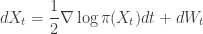
 as its equilibrium distribution. Informally, an SDE of this form is a continuous time process with infinitesimal transition kernel
 , the SDE
 on a common scale.


 is just the vector of regression coefficients,
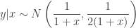
  . We assumed independent mean zero normal priors for the components of this vector, so the log prior is just the sum of logs of normal densities. Many scientific libraries will have built-in functions for returning the log-pdf of standard distributions, but if an explicit form is required, the log of the density of a
  at
at  is just
 , the likelihood associated with observation
  is
is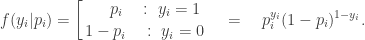
 we have
 observations gives the log likelihood
 is the linear predictor, so
  , giving
![\displaystyle \ell(\beta;y) = y^\textsf{T}X\beta - \mathbf{1}^\textsf{T}\log(\mathbf{1}+\exp[X\beta]).](https://s0.wp.com/latex.php?latex=%5Cdisplaystyle+%5Cell%28%5Cbeta%3By%29+%3D+y%5E%5Ctextsf%7BT%7DX%5Cbeta+-+%5Cmathbf%7B1%7D%5E%5Ctextsf%7BT%7D%5Clog%28%5Cmathbf%7B1%7D%2B%5Cexp%5BX%5Cbeta%5D%29.+&bg=ffffff&fg=333333&s=0&c=20201002)
 is 1 for success and -1 for failure. This isn’t really a problem, since the two encodings are related by
  . This new encoding is convenient in the context of a logit parameterisation since then

![\displaystyle \ell(\eta;\tilde y) = -\mathbf{1}\cdot \log(\mathbf{1}+\exp[-\tilde y\circ \eta]),](https://s0.wp.com/latex.php?latex=%5Cdisplaystyle+%5Cell%28%5Ceta%3B%5Ctilde+y%29+%3D+-%5Cmathbf%7B1%7D%5Ccdot+%5Clog%28%5Cmathbf%7B1%7D%2B%5Cexp%5B-%5Ctilde+y%5Ccirc+%5Ceta%5D%29%2C+&bg=ffffff&fg=333333&s=0&c=20201002)
 denotes the
 ![\displaystyle \ell(\beta;\tilde y) = -\mathbf{1}^\textsf{T} \log(\mathbf{1}+\exp[-\tilde y\circ X\beta]).](https://s0.wp.com/latex.php?latex=%5Cdisplaystyle+%5Cell%28%5Cbeta%3B%5Ctilde+y%29+%3D+-%5Cmathbf%7B1%7D%5E%5Ctextsf%7BT%7D+%5Clog%28%5Cmathbf%7B1%7D%2B%5Cexp%5B-%5Ctilde+y%5Ccirc+X%5Cbeta%5D%29.+&bg=ffffff&fg=333333&s=0&c=20201002)
![\displaystyle \ell(\beta; y) = -\mathbf{1}^\textsf{T} \log(\mathbf{1}+\exp[-(2y-\mathbf{1})\circ (X\beta)]),](https://s0.wp.com/latex.php?latex=%5Cdisplaystyle+%5Cell%28%5Cbeta%3B+y%29+%3D+-%5Cmathbf%7B1%7D%5E%5Ctextsf%7BT%7D+%5Clog%28%5Cmathbf%7B1%7D%2B%5Cexp%5B-%282y-%5Cmathbf%7B1%7D%29%5Ccirc+%28X%5Cbeta%29%5D%29%2C+&bg=ffffff&fg=333333&s=0&c=20201002)
