This blog post is derived from a computer practical session that I ran as part of my new course on Statistics for Big Data, previously discussed. This course covered a lot of material very quickly. In particular, I deferred introducing notions of hierarchical modelling until the Bayesian part of the course, where I feel it is more natural and powerful. However, some of the terminology associated with hierarchical statistical modelling probably seems a bit mysterious to those without a strong background in classical statistical modelling, and so this practical session was intended to clear up some potential confusion. I will analyse a simple one-way Analysis of Variance (ANOVA) model from a Bayesian perspective, making sure to highlight the difference between fixed and random effects in a Bayesian context where everything is random, as well as emphasising the associated identifiability issues. R code is used to illustrate the ideas.
Example scenario
We will consider the body mass index (BMI) of new male undergraduate students at a selection of UK Universities. Let us suppose that our data consist of measurements of (log) BMI for a random sample of 1,000 males at each of 8 Universities. We are interested to know if there are any differences between the Universities. Again, we want to model the process as we would simulate it, so thinking about how we would simulate such data is instructive. We start by assuming that the log BMI is a normal random quantity, and that the variance is common across the Universities in question (this is quite a big assumption, and it is easy to relax). We assume that the mean of this normal distribution is University-specific, but that we do not have strong prior opinions regarding the way in which the Universities differ. That said, we expect that the Universities would not be very different from one another.
Simulating data
A simple simulation of the data with some plausible parameters can be carried out as follows.
set.seed(1)
Z=matrix(rnorm(1000*8,3.1,0.1),nrow=8)
RE=rnorm(8,0,0.01)
X=t(Z+RE)
colnames(X)=paste("Uni",1:8,sep="")
Data=stack(data.frame(X))
boxplot(exp(values)~ind,data=Data,notch=TRUE)
Make sure that you understand exactly what this code is doing before proceeding. The boxplot showing the simulated data is given below.

Frequentist analysis
We will start with a frequentist analysis of the data. The model we would like to fit is
where i is an indicator for the University and j for the individual within a particular University. The “effect”, 
> mod=lm(values~ind,data=Data)
> summary(mod)

Call:
lm(formula = values ~ ind, data = Data)

Residuals:
     Min       1Q   Median       3Q      Max
-0.36846 -0.06778 -0.00069  0.06910  0.38219

Coefficients:
             Estimate Std. Error t value Pr(>|t|)
(Intercept)  3.101068   0.003223 962.244  < 2e-16 ***
indUni2     -0.006516   0.004558  -1.430 0.152826
indUni3     -0.017168   0.004558  -3.767 0.000166 ***
indUni4      0.017916   0.004558   3.931 8.53e-05 ***
indUni5     -0.022838   0.004558  -5.011 5.53e-07 ***
indUni6     -0.001651   0.004558  -0.362 0.717143
indUni7      0.007935   0.004558   1.741 0.081707 .
indUni8      0.003373   0.004558   0.740 0.459300
---
Signif. codes:  0 ‘***’ 0.001 ‘**’ 0.01 ‘*’ 0.05 ‘.’ 0.1 ‘ ’ 1

Residual standard error: 0.1019 on 7992 degrees of freedom
Multiple R-squared:  0.01439,	Adjusted R-squared:  0.01353
F-statistic: 16.67 on 7 and 7992 DF,  p-value: < 2.2e-16
We see that R has handled the identifiability problem using “treatment contrasts”, dropping the fixed effect for the first university, so that the intercept actually represents the mean value for the first University, and the effects for the other Univeristies represent the differences from the first University. If we would prefer to impose a sum constraint, then we can switch to sum contrasts with
options(contrasts=rep("contr.sum",2))
and then re-fit the model.
> mods=lm(values~ind,data=Data)
> summary(mods)

Call:
lm(formula = values ~ ind, data = Data)

Residuals:
     Min       1Q   Median       3Q      Max
-0.36846 -0.06778 -0.00069  0.06910  0.38219

Coefficients:
              Estimate Std. Error  t value Pr(>|t|)
(Intercept)  3.0986991  0.0011394 2719.558  < 2e-16 ***
ind1         0.0023687  0.0030146    0.786 0.432048
ind2        -0.0041477  0.0030146   -1.376 0.168905
ind3        -0.0147997  0.0030146   -4.909 9.32e-07 ***
ind4         0.0202851  0.0030146    6.729 1.83e-11 ***
ind5        -0.0204693  0.0030146   -6.790 1.20e-11 ***
ind6         0.0007175  0.0030146    0.238 0.811889
ind7         0.0103039  0.0030146    3.418 0.000634 ***
---
Signif. codes:  0 ‘***’ 0.001 ‘**’ 0.01 ‘*’ 0.05 ‘.’ 0.1 ‘ ’ 1

Residual standard error: 0.1019 on 7992 degrees of freedom
Multiple R-squared:  0.01439,	Adjusted R-squared:  0.01353
F-statistic: 16.67 on 7 and 7992 DF,  p-value: < 2.2e-16
This has 7 degrees of freedom for the effects, as before, but ensures that the 8 effects sum to precisely zero. This is arguably more interpretable in this case.
Bayesian analysis
We will now analyse the simulated data from a Bayesian perspective, using JAGS.
Fixed effects
All parameters in Bayesian models are uncertain, and therefore random, so there is much confusion regarding the difference between “fixed” and “random” effects in a Bayesian context. For “fixed” effects, our prior captures the idea that we sample the effects independently from a “fixed” (typically vague) prior distribution. We could simply code this up and fit it in JAGS as follows.
require(rjags)
n=dim(X)[1]
p=dim(X)[2]
data=list(X=X,n=n,p=p)
init=list(mu=2,tau=1)
modelstring="
  model {
    for (j in 1:p) {
      theta[j]~dnorm(0,0.0001)
      for (i in 1:n) {
        X[i,j]~dnorm(mu+theta[j],tau)
      }
    }
    mu~dnorm(0,0.0001)
    tau~dgamma(1,0.0001)
  }
"
model=jags.model(textConnection(modelstring),data=data,inits=init)
update(model,n.iter=1000)
output=coda.samples(model=model,variable.names=c("mu","tau","theta"),n.iter=100000,thin=10)
print(summary(output))
plot(output)
autocorr.plot(output)
pairs(as.matrix(output))
crosscorr.plot(output)
On running the code we can clearly see that this naive approach leads to high posterior correlation between the mean and the effects, due to the fundamental lack of identifiability of the model. This also leads to MCMC mixing problems, but it is important to understand that this computational issue is conceptually entirely separate from the fundamental statisticial identifiability issue. Even if we could avoid MCMC entirely, the identifiability issue would remain.
A quick fix for the identifiability issue is to use “treatment contrasts”, just as for the frequentist model. We can implement that as follows.
data=list(X=X,n=n,p=p)
init=list(mu=2,tau=1)
modelstring="
  model {
    for (j in 1:p) {
      for (i in 1:n) {
        X[i,j]~dnorm(mu+theta[j],tau)
      }
    }
    theta[1]<-0
    for (j in 2:p) {
      theta[j]~dnorm(0,0.0001)
    }
    mu~dnorm(0,0.0001)
    tau~dgamma(1,0.0001)
  }
"
model=jags.model(textConnection(modelstring),data=data,inits=init)
update(model,n.iter=1000)
output=coda.samples(model=model,variable.names=c("mu","tau","theta"),n.iter=100000,thin=10)
print(summary(output))
plot(output)
autocorr.plot(output)
pairs(as.matrix(output))
crosscorr.plot(output)
Running this we see that the model now works perfectly well, mixes nicely, and gives sensible inferences for the treatment effects.
Another source of confusion for models of this type is data formating and indexing in JAGS models. For our balanced data there was not problem passing in data to JAGS as a matrix and specifying the model using nested loops. However, for unbalanced designs this is not necessarily so convenient, and so then it can be helpful to specify the model based on two-column data, as we would use for fitting using lm(). This is illustrated with the following model specification, which is exactly equivalent to the previous model, and should give identical (up to Monte Carlo error) results.
N=n*p
data=list(y=Data$values,g=Data$ind,N=N,p=p)
init=list(mu=2,tau=1)
modelstring="
  model {
    for (i in 1:N) {
      y[i]~dnorm(mu+theta[g[i]],tau)
    }
    theta[1]<-0
    for (j in 2:p) {
      theta[j]~dnorm(0,0.0001)
    }
    mu~dnorm(0,0.0001)
    tau~dgamma(1,0.0001)
  }
"
model=jags.model(textConnection(modelstring),data=data,inits=init)
update(model,n.iter=1000)
output=coda.samples(model=model,variable.names=c("mu","tau","theta"),n.iter=100000,thin=10)
print(summary(output))
plot(output)
As suggested above, this indexing scheme is much more convenient for unbalanced data, and hence widely used. However, since our data is balanced here, we will revert to the matrix approach for the remainder of the post.
One final thing to consider before moving on to random effects is the sum-contrast model. We can implement this in various ways, but I’ve tried to encode it for maximum clarity below, imposing the sum-to-zero constraint via the final effect.
data=list(X=X,n=n,p=p)
init=list(mu=2,tau=1)
modelstring="
  model {
    for (j in 1:p) {
      for (i in 1:n) {
        X[i,j]~dnorm(mu+theta[j],tau)
      }
    }
    for (j in 1:(p-1)) {
      theta[j]~dnorm(0,0.0001)
    }
    theta[p] <- -sum(theta[1:(p-1)])
    mu~dnorm(0,0.0001)
    tau~dgamma(1,0.0001)
  }
"
model=jags.model(textConnection(modelstring),data=data,inits=init)
update(model,n.iter=1000)
output=coda.samples(model=model,variable.names=c("mu","tau","theta"),n.iter=100000,thin=10)
print(summary(output))
plot(output)
Again, this works perfectly well and gives similar results to the frequentist analysis.
Random effects
The key difference between fixed and random effects in a Bayesian framework is that random effects are not independent, being drawn from a distribution with parameters which are not fixed. Essentially, there is another level of hierarchy involved in the specification of the random effects. This is best illustrated by example. A random effects model for this problem is given below.
data=list(X=X,n=n,p=p)
init=list(mu=2,tau=1)
modelstring="
  model {
    for (j in 1:p) {
      theta[j]~dnorm(0,taut)
      for (i in 1:n) {
        X[i,j]~dnorm(mu+theta[j],tau)
      }
    }
    mu~dnorm(0,0.0001)
    tau~dgamma(1,0.0001)
    taut~dgamma(1,0.0001)
  }
"
model=jags.model(textConnection(modelstring),data=data,inits=init)
update(model,n.iter=1000)
output=coda.samples(model=model,variable.names=c("mu","tau","taut","theta"),n.iter=100000,thin=10)
print(summary(output))
plot(output)
The only difference between this and our first naive attempt at a Bayesian fixed effects model is that we have put a gamma prior on the precision of the effect. Note that this model now runs and fits perfectly well, with reasonable mixing, and gives sensible parameter inferences. Although the effects here are not constrained to sum-to-zero, like in the case of sum contrasts for a fixed effects model, the prior encourages shrinkage towards zero, and so the random effect distribution can be thought of as a kind of soft version of a hard sum-to-zero constraint. From a predictive perspective, this model is much more powerful. In particular, using a random effects model, we can make strong predictions for unobserved groups (eg. a ninth University), with sensible prediction intervals based on our inferred understanding of how similar different universities are. Using a fixed effects model this isn’t really possible. Even for a Bayesian version of a fixed effects model using proper (but vague) priors, prediction intervals for unobserved groups are not really sensible.
Since we have used simulated data here, we can compare the estimated random effects with the true effects generated during the simulation.
> apply(as.matrix(output),2,mean)
           mu           tau          taut      theta[1]      theta[2]
 3.098813e+00  9.627110e+01  7.015976e+03  2.086581e-03 -3.935511e-03
     theta[3]      theta[4]      theta[5]      theta[6]      theta[7]
-1.389099e-02  1.881528e-02 -1.921854e-02  5.640306e-04  9.529532e-03
     theta[8]
 5.227518e-03
> RE
[1]  0.002637034 -0.008294518 -0.014616348  0.016839902 -0.015443243
[6] -0.001908871  0.010162117  0.005471262
We see that the Bayesian random effects model has done an excellent job of estimation. If we wished, we could relax the assumption of common variance across the groups by making tau a vector indexed by j, though there is not much point in persuing this here, since we know that the groups do all have the same variance.
Strong subjective priors
The above is the usual story regarding fixed and random effects in Bayesian inference. I hope this is reasonably clear, so really I should quit while I’m ahead… However, the issues are really a bit more subtle than I’ve suggested. The inferred precision of the random effects was around 7,000, so now lets re-run the original, naive, “fixed effects” model with a strong subjective Bayesian prior on the distribution of the effects.
data=list(X=X,n=n,p=p)
init=list(mu=2,tau=1)
modelstring="
  model {
    for (j in 1:p) {
      theta[j]~dnorm(0,7000)
      for (i in 1:n) {
        X[i,j]~dnorm(mu+theta[j],tau)
      }
    }
    mu~dnorm(0,0.0001)
    tau~dgamma(1,0.0001)
  }
"
model=jags.model(textConnection(modelstring),data=data,inits=init)
update(model,n.iter=1000)
output=coda.samples(model=model,variable.names=c("mu","tau","theta"),n.iter=100000,thin=10)
print(summary(output))
plot(output)
This model also runs perfectly well and gives sensible inferences, despite the fact that the effects are iid from a fixed distribution and there is no hard constraint on the effects. Similarly, we can make sensible predictions, together with appropriate prediction intervals, for an unobserved group. So it isn’t so much the fact that the effects are coupled via an extra level of hierarchy that makes things work. It’s really the fact that the effects are sensibly distributed and not just sampled directly from a vague prior. So for “real” subjective Bayesians the line between fixed and random effects is actually very blurred indeed…
![t\in [0,1]](https://s0.wp.com/latex.php?latex=t%5Cin+%5B0%2C1%5D&bg=ffffff&fg=333333&s=0&c=20201002) we define
we define![\pi_t(\theta|y) \propto \pi(\theta|y)^t \propto [ \pi(\theta)\pi(y|\theta) ]^t.](https://s0.wp.com/latex.php?latex=%5Cpi_t%28%5Ctheta%7Cy%29+%5Cpropto+%5Cpi%28%5Ctheta%7Cy%29%5Et+%5Cpropto+%5B+%5Cpi%28%5Ctheta%29%5Cpi%28y%7C%5Ctheta%29+%5D%5Et.&bg=ffffff&fg=333333&s=0&c=20201002)
 and tend to a flat distribution as
  . However, for Bayesian posterior distributions, there is a different way of tempering that is often more natural and useful, and that is to temper using the power posterior, defined by
 . Thus, the family of distributions forms a natural bridge or path from the prior to the posterior distributions. The power posterior is a special case of the more general concept of a geometric path from distribution
  (at
(at  (at
(at 
 is the prior and
  is the posterior.
 mixing will be good, as prior-like distributions are usually well-behaved, and the mixing of these "high temperature" chains can help to improve the mixing of the "low temperature" chains that are more like the posterior (note that
![\pi(y) = E_\pi [ \pi(y|\theta) ]](https://s0.wp.com/latex.php?latex=%5Cpi%28y%29+%3D+E_%5Cpi+%5B+%5Cpi%28y%7C%5Ctheta%29+%5D&bg=ffffff&fg=333333&s=0&c=20201002)
 , we can construct the Monte Carlo estimate
 th chain
  , so that
  and
and  , then we can write the evidence in telescoping fashion as
 , which can be estimated using the output from the
  th chain(s). Again, this can be done in a variety of ways, using your favourite bridge sampling estimator, but the point is that the estimator should be reasonably good due to the fact that the
![\displaystyle \mbox{}\qquad = E_i\left[\pi(y|\theta)^{t_{i+1}-t_i}\right],](https://s0.wp.com/latex.php?latex=%5Cdisplaystyle+%5Cmbox%7B%7D%5Cqquad+%3D+E_i%5Cleft%5B%5Cpi%28y%7C%5Ctheta%29%5E%7Bt_%7Bi%2B1%7D-t_i%7D%5Cright%5D%2C&bg=ffffff&fg=333333&s=0&c=20201002)
![\displaystyle \log\pi(y) = \sum_{i=0}^{N-1} \log\frac{z_{i+1}}{z_i} = \sum_{i=0}^{N-1} \log E_i\left[\pi(y|\theta)^{t_{i+1}-t_i}\right]](https://s0.wp.com/latex.php?latex=%5Cdisplaystyle+%5Clog%5Cpi%28y%29+%3D+%5Csum_%7Bi%3D0%7D%5E%7BN-1%7D+%5Clog%5Cfrac%7Bz_%7Bi%2B1%7D%7D%7Bz_i%7D+%3D+%5Csum_%7Bi%3D0%7D%5E%7BN-1%7D+%5Clog+E_i%5Cleft%5B%5Cpi%28y%7C%5Ctheta%29%5E%7Bt_%7Bi%2B1%7D-t_i%7D%5Cright%5D&bg=ffffff&fg=333333&s=0&c=20201002)
![\displaystyle = \sum_{i=0}^{N-1} \log E_i\left[\exp\{(t_{i+1}-t_i)\log\pi(y|\theta)\}\right].\qquad(\dagger)](https://s0.wp.com/latex.php?latex=%5Cdisplaystyle+%3D+%5Csum_%7Bi%3D0%7D%5E%7BN-1%7D+%5Clog+E_i%5Cleft%5B%5Cexp%5C%7B%28t_%7Bi%2B1%7D-t_i%29%5Clog%5Cpi%28y%7C%5Ctheta%29%5C%7D%5Cright%5D.%5Cqquad%28%5Cdagger%29&bg=ffffff&fg=333333&s=0&c=20201002)
 and
and  are sufficiently close, it will be approximately OK to switch the expectation and exponential, giving
![\displaystyle \log\pi(y) \approx \sum_{i=0}^{N-1}(t_{i+1}-t_i)E_i\left[\log\pi(y|\theta)\right].](https://s0.wp.com/latex.php?latex=%5Cdisplaystyle+%5Clog%5Cpi%28y%29+%5Capprox+%5Csum_%7Bi%3D0%7D%5E%7BN-1%7D%28t_%7Bi%2B1%7D-t_i%29E_i%5Cleft%5B%5Clog%5Cpi%28y%7C%5Ctheta%29%5Cright%5D.&bg=ffffff&fg=333333&s=0&c=20201002)
![\displaystyle \log\pi(y) = \int_0^1 E_t\left[\log\pi(y|\theta)\right]dt.](https://s0.wp.com/latex.php?latex=%5Cdisplaystyle+%5Clog%5Cpi%28y%29+%3D+%5Cint_0%5E1+E_t%5Cleft%5B%5Clog%5Cpi%28y%7C%5Ctheta%29%5Cright%5Ddt.&bg=ffffff&fg=333333&s=0&c=20201002)
 directly, since there there is no numerical integration error to worry about.
 . Here it isn’t obvious why we’d want to know that, but we’ll compute it anyway to illustrate the method. As before, we expand as a telescopic product, where the
 ![\displaystyle \frac{z_{i+1}}{z_i} = E_i\left[\exp\{-(\gamma_{i+1}-\gamma_i)(x^2-1)^2\}\right].](https://s0.wp.com/latex.php?latex=%5Cdisplaystyle+%5Cfrac%7Bz_%7Bi%2B1%7D%7D%7Bz_i%7D+%3D+E_i%5Cleft%5B%5Cexp%5C%7B-%28%5Cgamma_%7Bi%2B1%7D-%5Cgamma_i%29%28x%5E2-1%29%5E2%5C%7D%5Cright%5D.&bg=ffffff&fg=333333&s=0&c=20201002)
 . A complete R script to run the Metropolis coupled sampler and compute the evidence is given below.
 from the prior and then sampling a corresponding data set
  from the model. This simulated data set is compared with the true data
  using some (pseudo-)norm,
  , and accepting
  . It should be clear that if we are using a proper norm then as
  tends to zero the distribution of the accepted values tends to the desired posterior distribution of the parameters given the data.
 for
for  , then it should be clear that replacing the acceptance criterion with
  will also lead to a scheme tending to the true posterior as
 , and a forwards-simulation model for the data
  . It is clear that a simple algorithm for simulating from the desired posterior
  can be obtained as follows. First simulate from the joint distribution
  by simulating
  and then
  . This gives a sample
  from the joint distribution. A simple rejection algorithm which rejects the proposed pair unless

 , keep
  , keep
 (ideally a sufficient statistic), and accepting provided that
  for some suitable choice of metric and
  . Note that I have deliberately adopted a functional programming style, making use of the lapply function for the most computationally intensive steps. The reason for this will soon become apparent. Note that rather than pre-specifying a cutoff
 is an
is an  matrix. The idea of variable selection is that probably not all of the p covariates are useful for predicting y, and therefore it would be useful to identify the variables which are, and just use those. Clearly each combination of variables corresponds to a different model, and so the variable selection amounts to choosing among the
  possible models. For large values of p it won’t be practical to consider each possible model separately, and so the idea of Bayesian variable selection is to consider a model containing all of the possible model combinations as sub-models, and the variable selection problem as just another aspect of the model which must be estimated from data. I’m simplifying and glossing over lots of details here, but there is a very nice review paper by
  for each covariate, and introduce these into the model in order to “zero out” inactive covariates. That is we write the ith regression coefficient
  as
as  , so that
  is the regression coefficient when
  , and “doesn’t matter” when
  . There are various ways to choose the prior over
 and
and  of the form
 , of the form
 . On the other hand, the PMMH algorithm is an MCMC algorithm which targets the full joint posterior distribution
  . Now, the PMMH scheme does reduce to the pseudo-marginal scheme if samples of
  ). Below I will describe the algorithm and explain why it works, but first it is necessary to understand the relationship between marginal, joint and “likelihood-free” MCMC updating schemes for such latent variable models.
 and accepted with probability
  , where
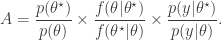
 required in the acceptance ratio is often difficult to compute.
 even when we can’t evaluate it, or marginalise
  . The pair
 . The pair
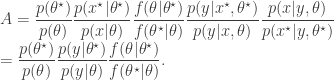
 , as the algorithms above. First, a proposed new
  is generated by running a bootstrap particle filter (as described in the previous post, and below) using the proposed new model parameters,
  is accepted using the Metropolis-Hastings ratio
 is the particle filter’s (unbiased) estimate of marginal likelihood, described in the previous post, and below. Note that this approach tends to the perfect joint/marginal updating scheme as the number of particles used in the filter tends to infinity. Note also that for a single particle, the particle filter just blindly forward simulates from
  and that the filter’s estimate of marginal likelihood is just the observed data likelihood
  leading precisely to the simple likelihood-free scheme. To understand for an arbitrary finite number of particles,
  , one needs to think carefully about the structure of the particle filter.
 ,
,  ,
,  . Initialise the particle filter with
  , where
  and
and  (note that
  is undefined). Now suppose at time
  :
:  . First resample by sampling
  ,
,  . Here we use
  for the discrete distribution on
  with probability mass function
  . Next sample
  . Set
. Set 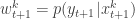 and
and 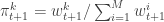 . Finally, propagate
  to the next step… We define the filter’s estimate of likelihood as
 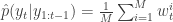 and
and 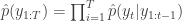 . See
. See ![\displaystyle \tilde{q}(\mathbf{x}_0,\ldots,\mathbf{x}_T,\mathbf{a}_0,\ldots,\mathbf{a}_{T-1}) = \left[\prod_{k=1}^M p(x_0^k)\right] \left[\prod_{t=0}^{T-1} \prod_{k=1}^M \pi_t^{a_t^k} p(x_{t+1}^k|x_t^{a_t^k}) \right]](https://s0.wp.com/latex.php?latex=%5Cdisplaystyle++%5Ctilde%7Bq%7D%28%5Cmathbf%7Bx%7D_0%2C%5Cldots%2C%5Cmathbf%7Bx%7D_T%2C%5Cmathbf%7Ba%7D_0%2C%5Cldots%2C%5Cmathbf%7Ba%7D_%7BT-1%7D%29++%3D+%5Cleft%5B%5Cprod_%7Bk%3D1%7D%5EM+p%28x_0%5Ek%29%5Cright%5D+%5Cleft%5B%5Cprod_%7Bt%3D0%7D%5E%7BT-1%7D++++%5Cprod_%7Bk%3D1%7D%5EM+%5Cpi_t%5E%7Ba_t%5Ek%7D+p%28x_%7Bt%2B1%7D%5Ek%7Cx_t%5E%7Ba_t%5Ek%7D%29+%5Cright%5D++&bg=ffffff&fg=333333&s=0&c=20201002)
 from
from  giving the joint density

 , and
, and  . If we now think about the structure of the PMMH algorithm, our proposal on the space of all random variables in the problem is in fact

 when we consider just the parameters and the selected trajectory. But if we consider the terms in the joint distribution of the proposal corresponding to the trajectory selected by
 ![\displaystyle p_\theta(x_0^{b_0^{k'}})\left[\prod_{t=0}^{T-1} \pi_t^{b_t^{k'}} p_\theta(x_{t+1}^{b_{t+1}^{k'}}|x_t^{b_t^{k'}})\right]\pi_T^{k'} = p_\theta(x_{0:T}^{k'})\prod_{t=0}^T \pi_t^{b_t^{k'}}](https://s0.wp.com/latex.php?latex=%5Cdisplaystyle++p_%5Ctheta%28x_0%5E%7Bb_0%5E%7Bk%27%7D%7D%29%5Cleft%5B%5Cprod_%7Bt%3D0%7D%5E%7BT-1%7D+%5Cpi_t%5E%7Bb_t%5E%7Bk%27%7D%7D++++p_%5Ctheta%28x_%7Bt%2B1%7D%5E%7Bb_%7Bt%2B1%7D%5E%7Bk%27%7D%7D%7Cx_t%5E%7Bb_t%5E%7Bk%27%7D%7D%29%5Cright%5D%5Cpi_T%5E%7Bk%27%7D++%3D++p_%5Ctheta%28x_%7B0%3AT%7D%5E%7Bk%27%7D%29%5Cprod_%7Bt%3D0%7D%5ET+%5Cpi_t%5E%7Bb_t%5E%7Bk%27%7D%7D++&bg=ffffff&fg=333333&s=0&c=20201002)
 in terms of the unnormalised weights, simplifies to
 in the acceptance ratio, we knock out the normalising constant, allowing all of the other terms in the proposal to be marginalised away. In other words, the target of the chain can be written as proportional to