Introduction to the particle Gibbs sampler

Introduction

Particle MCMC (the use of approximate SMC proposals within exact MCMC algorithms) is arguably one of the most important developments in computational Bayesian inference of the 21st Century. The key concepts underlying these methods are described in a famously impenetrable “read paper” by Andrieu et al (2010). Probably the most generally useful method outlined in that paper is the particle marginal Metropolis-Hastings (PMMH) algorithm that I have described previously – that post is required preparatory reading for this one.

In this post I want to discuss some of the other topics covered in the pMCMC paper, leading up to a description of the particle Gibbs sampler. The basic particle Gibbs algorithm is arguably less powerful than PMMH for a few reasons, some of which I will elaborate on. But there is still a lot of active research concerning particle Gibbs-type algorithms, which are attempting to address some of the deficiencies of the basic approach. Clearly, in order to understand and appreciate the recent developments it is first necessary to understand the basic principles, and so that is what I will concentrate on here. I’ll then finish with some pointers to more recent work in this area.

PIMH

I will adopt the same approach and notation as for my post on the PMMH algorithm, using a simple bootstrap particle filter for a state space model as the SMC proposal. It is simplest to understand particle Gibbs first in the context of known static parameters, and so it is helpful to first reconsider the special case of the PMMH algorithm where there are no unknown parameters and only the state path, $x$ of the process is being updated. That is, we target $p(x|y)$ (for known, fixed, $\theta$ ) rather than $p(\theta,x|y)$ . This special case is known as the particle independent Metropolis-Hastings (PIMH) sampler.

Here we envisage proposing a new path $x_{0:T}^\star$ using a bootstrap filter, and then accepting the proposal with probability $\min\{1,A\}$ , where $A$ is the Metropolis-Hastings ratio

$\displaystyle A = \frac{\hat{p}(y_{1:T})^\star}{\hat{p}(y_{1:T})},$

where $\hat{p}(y_{1:T})^\star$ is the bootstrap filter’s estimate of marginal likelihood for the new path, and $\hat{p}(y_{1:T})$ is the estimate associated with the current path. Again using notation from the previous post it is clear that this ratio targets a distribution on the joint space of all simulated random variables proportional to

$\displaystyle \hat{p}(y_{1:T})\tilde{q}(\mathbf{x}_0,\ldots,\mathbf{x}_T,\mathbf{a}_0,\ldots,\mathbf{a}_{T-1})$

and that in this case the marginal distribution of the accepted path is exactly $p(x_{0:T}|y_{1:T})$ . Again, be sure to see the previous post for the explanation.

Conditional SMC update

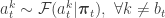
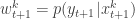
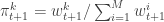
So far we have just recapped the previous post in the case of known parameters, but it gives us insight in how to proceed. A general issue with Metropolis independence samplers in high dimensions is that they often exhibit “sticky” behaviour, whereby an unusually “good” accepted path is hard to displace. This motivates consideration of a block-Gibbs-style algorithm where updates are used that are always accepted. It is clear that simply running a bootstrap filter will target the particle filter distribution

$\tilde{q}(\mathbf{x}_0,\ldots,\mathbf{x}_T,\mathbf{a}_0,\ldots,\mathbf{a}_{T-1})$

and so the marginal distribution of the accepted path will be the approximate $\hat{p}(x_{0:T}|y_{1:T})$ rather than the exact conditional distribution $p(x_{0:T}|y_{1:T})$ . However, we know from consideration of the PIMH algorithm that what we really want to do is target the slightly modified distribution proportional to

$\displaystyle \hat{p}(y_{1:T})\tilde{q}(\mathbf{x}_0,\ldots,\mathbf{x}_T,\mathbf{a}_0,\ldots,\mathbf{a}_{T-1})$ ,

as this will lead to accepted paths with the exact marginal distribution. For the PIMH this modification is achieved using a Metropolis-Hastings correction, but we now try to avoid this by instead conditioning on the previously accepted path. For this target the accepted paths have exactly the required marginal distribution, so we now write the target as the product of the marginal for the current path times a conditional for all of the remaining variables.

$\displaystyle \frac{p(x_{0:T}^k|y_{1:T})}{M^T} \times \frac{M^T}{p(x_{0:T}^k|y_{1:T})} \hat{p}(y_{1:T})\tilde{q}(\mathbf{x}_0,\ldots,\mathbf{x}_T,\mathbf{a}_0,\ldots,\mathbf{a}_{T-1})$

where in addition to the correct marginal for $x$ we assume iid uniform ancestor indices. The important thing to note here is that the conditional distribution of the remaining variables simplifies to

$\displaystyle \frac{\tilde{q}(\mathbf{x}_0,\ldots,\mathbf{x}_T,\mathbf{a}_0,\ldots,\mathbf{a}_{T-1})} {\displaystyle p(x_0^{b_0^k})\left[\prod_{t=0}^{T-1} \pi_t^{b_t^k}p\left(x_{t+1}^{b_{t+1}^k}|x_t^{b_t^k}\right)\right]}$ .

The terms in the denominator are precisely the terms in the numerator corresponding to the current path, and hence “cancel out” the current path terms in the numerator. It is therefore clear that we can sample directly from this conditional distribution by running a bootstrap particle filter that includes the current path and which leaves the current path fixed. This is the conditional SMC (CSMC) update, which here is just a conditional bootstrap particle filter update. It is clear from the form of the conditional density how this filter must be constructed, but for completeness it is described below.

The bootstrap filter is run conditional on one trajectory. This is usually the trajectory sampled at the last run of the particle filter. The idea is that you do not sample new state or ancestor values for that one trajectory. Note that this guarantees that the conditioned on trajectory survives the filter right through to the final sweep of the filter at which point a new trajectory is picked from the current selection of $M$ paths, of which the conditioned-on trajectory is one.

Let $x_{1:T} = (x_1^{b_1},x_2^{b_2},\ldots,x_T^{b_T})$ be the path that is to be conditioned on, with ancestral lineage $b_{1:T}$ . Then, for $k\not= b_1$ , sample $x_0^k \sim p(x_0)$ and set $\pi_0^k=1/M$ . Now suppose that at time $t$ we have a weighted sample from $p(x_t|y_{1:t})$ . First resample by sampling $a_t^k\sim \mathcal{F}(a_t^k|\boldsymbol{\pi}_t),\ \forall k\not= b_t$ . Next sample $x_{t+1}^k\sim p(x_{t+1}^k|x_t^{a_t^k}),\ \forall k\not=b_t$ . Then for all $k$ set $w_{t+1}^k=p(y_{t+1}|x_{t+1}^k)$ and normalise with $\pi_{t+1}^k=w_{t+1}^k/\sum_{i=1}^M w_{t+1}^i$ . Propagate this weighted set of particles to the next time point. At time $T$ select a single trajectory by sampling $k'\sim \mathcal{F}(k'|\boldsymbol{\pi}_T)$ .

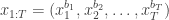
This defines a block Gibbs sampler which updates $2(M-1)T+1$ of the $2MT+1$ random variables in the augmented state space at each iteration. Since the block of variables to be updated is random, this defines an ergodic sampler for $M\geq2$ particles, and we have explained why the marginal distribution of the selected trajectory is the exact conditional distribution.

Before going on to consider the introduction of unknown parameters, it is worth considering the limitations of this method. One of the main motivations for considering a Gibbs-style update was concern about the “stickiness” of a Metropolis independence sampler. However, it is clear that conditional SMC updates also have the potential to stick. For a large number of time points, particle filter genealogies coalesce, or degenerate, to a single path. Since here we are conditioning on the current path, if there is coalescence, it is guaranteed to be to the previous path. So although the conditional SMC updates are always accepted, it is likely that much of the new path will be identical to the previous path, which is just another kind of “sticking” of the sampler. This problem with conditional SMC and particle Gibbs more generally is well recognised, and quite a bit of recent research activity in this area is directed at alleviating this sticking problem. The most obvious strategy to use is “backward sampling” (Godsill et al, 2004), which has been used in this context by Lindsten and Schon (2012), Whiteley et al (2010), and Chopin and Singh (2013), among others. Another related idea is “ancestor sampling” (Lindsten et al, 2014), which can be done in a single forward pass. Both of these techniques work well, but both rely on the tractability of the transition kernel of the state space model, which can be problematic in certain applications.

Particle Gibbs sampling

As we are working in the context of Gibbs-style updates, the introduction of static parameters, $\theta$ , into the problem is relatively straightforward. It turns out to be correct to do the obvious thing, which is to alternate between sampling $\theta$ given $y$ and the currently sampled path, $x$ , and sampling a new path using a conditional SMC update, conditional on the previous path in addition to $\theta$ and $y$ . Although this is the obvious thing to do, understanding exactly why it works is a little delicate, due to the augmented state space and conditional SMC update. However, it is reasonably clear that this strategy defines a “collapsed Gibbs sampler” (Lui, 1994), and so actually everything is fine. This particular collapsed Gibbs sampler is relatively easy to understand as a marginal sampler which integrates out the augmented variables, but then nevertheless samples the augmented variables at each iteration conditional on everything else.

Note that the Gibbs update of $\theta$ may be problematic in the context of a state space model with intractable transition kernel.

In a subsequent post I’ll show how to code up the particle Gibbs and other pMCMC algorithms in a reasonably efficient way.

References

Andrieu, Christophe, Arnaud Doucet, and Roman Holenstein. “Particle Markov chain Monte Carlo methods.” Journal of the Royal Statistical Society: Series B (Statistical Methodology) 72.3 (2010): 269-342.
Chopin, Nicolas, and Sumeetpal S. Singh. “On the particle Gibbs sampler.” arXiv preprint arXiv:1304.1887 (2013).
Godsill, Simon J., Arnaud Doucet, and Mike West. “Monte Carlo smoothing for nonlinear time series.” Journal of the American Statistical Association 99.465 (2004).
Lindsten, Fredrik, and Thomas B. Schön. “On the use of backward simulation in the particle Gibbs sampler.” Acoustics, Speech and Signal Processing (ICASSP), 2012 IEEE International Conference on. IEEE, 2012.
Lindsten, Fredrik, Michael I. Jordan, and Thomas B. Schön. “Particle Gibbs with Ancestor Sampling.” arXiv preprint arXiv:1401.0604 (2014).
Liu, Jun S. “The collapsed Gibbs sampler in Bayesian computations with applications to a gene regulation problem.” Journal of the American Statistical Association 89.427 (1994): 958-966.
Whiteley, Nick, Christophe Andrieu, and Arnaud Doucet. “Efficient Bayesian inference for switching state-space models using discrete particle Markov chain Monte Carlo methods.” arXiv preprint arXiv:1011.2437 (2010).

2 thoughts on “Introduction to the particle Gibbs sampler”

Pingback: Index to first 50 posts | Darren Wilkinson's research blog
Kai Xu says:

05/10/2016 at 21:48

Hi Darren,

This post (along with its preparatory posts) is very helpful to learn PG. Really appreciate your work.

Near to the end of this post, can you please give a concrete example of “a state space model with intractable transition kernel”?

Kai

Introduction to the particle Gibbs sampler

Introduction

PIMH

Conditional SMC update

Particle Gibbs sampling

References

Published by

darrenjw

2 thoughts on “Introduction to the particle Gibbs sampler”

Leave a comment Cancel reply

Introduction

PIMH

Conditional SMC update

Particle Gibbs sampling

References

Share this:

Related

Published by

darrenjw

2 thoughts on “Introduction to the particle Gibbs sampler”

Leave a comment Cancel reply