Metropolis-Hastings MCMC algorithms

Background

Over the next few months I’m intending to have a series of posts on recent developments in MCMC and algorithms of Metropolis-Hastings type. These posts will assume a basic familiarity with stochastic simulation and R. For reference, I have some old notes on stochastic simulation and MCMC from a course I used to teach. There were a set of computer practicals associated with the course which focused on understanding the algorithms, mainly using R. Indeed, this post is going to make use of the example from this old practical. If anything about the rest of this post doesn’t make sense, you might need to review some of this background material. My favourite introductory text book on this subject is Gamerman’s Markov Chain Monte Carlo. In this post I’m going to briefly recap the key idea behind the Metropolis-Hastings algorithm, and illustrate how these kinds of algorithms are typically implemented. In order to keep things as simple as possible, I’m going to use R for implementation, but as discussed in a previous post, that probably won’t be a good idea for non-trivial applications.

Metropolis-Hastings

The motivation is a need to understand a complex probability distribution, p(x). In applications to Bayesian statistics, this distribution is usually a posterior from a Bayesian analysis. A good way to understand an intractable distribution is to simulate realisations from it and study those. However, this often isn’t easy, either. The idea behind MCMC is to simulate a Markov chain whose equilibrium distribution is p(x). Metropolis-Hastings (M-H) provides a way to correct a fairly arbitrary transition kernel q(x’|x) (which typically won’t have p(x) as its equilibrium) to give a chain which does have the desired target. In M-H, the transition kernel is used to generate a proposed new value, x’ for the chain, which is then accepted as the new state at random with a particular probability a(x’|x)=min(1,A), where A = p(x’)q(x|x’)/[p(x)q(x’|x)].

If the value is accepted, then the chain moves to the proposed new state, x’. If the value is not accepted, the chain still advances to the next step, but the new state is given by the previous state of the chain, x.

It is clear that this algorithm is also a Markov chain, and that for x’ != x, the transition kernel of this chain is q(x’|x)a(x’|x). A couple of lines of algebra will then confirm that this “corrected” Markov chain satisfies detailed balance for the target p(x). Therefore, under some regularity conditions, this chain will have p(x) as its equilibrium, and this gives a convenient way of simulating values from this target.

Special case: the Metropolis method

It is clear from the form of the acceptance probability that a considerable simplification arises in the case where the proposal kernel is symmetric, having q(x’|x)=q(x|x’). This is useful, as a convenient updating strategy is often to update the current value of x by adding an innovation sampled from a distribution that is symmetric about zero. This clearly gives a symmetric kernel, which then drops out of the acceptance ratio, to give A=p(x’)/p(x).

Example

The example we will use for illustration is a Metropolis method for the standard normal distribution using innovations from a U(-eps,eps) distribution. Below is a simple R implementation of the algorithm

metrop1=function(n=1000,eps=0.5) 
{
        vec=vector("numeric", n)
        x=0
        vec[1]=x
        for (i in 2:n) {
                innov=runif(1,-eps,eps)
                can=x+innov
                aprob=min(1,dnorm(can)/dnorm(x))
                u=runif(1)
                if (u < aprob) 
                        x=can
                vec[i]=x
        }
        vec
}

First a candidate value (can) is constructed by perturbing the current state of the chain with the uniform innovation. Then the acceptance probability is computed, and the chain is updated appropriately depending on whether the proposed new value is accepted. Note the standard trick of picking an event with probability p by checking to see if u<p, where u is a draw from a U(0,1).

We can execute this code and plot the results with the following peice of code:

plot.mcmc<-function(mcmc.out)
{
	op=par(mfrow=c(2,2))
	plot(ts(mcmc.out),col=2)
	hist(mcmc.out,30,col=3)
	qqnorm(mcmc.out,col=4)
	abline(0,1,col=2)
	acf(mcmc.out,col=2,lag.max=100)
	par(op)
}

metrop.out<-metrop1(10000,1)
plot.mcmc(metrop.out)
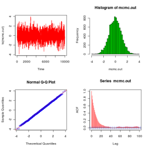
Plots showing convergence of the Markov chain to a N(0,1) equilibrium distribution

From these plots we see that the algorithm seems to be working as expected. Before finishing this post, it is worth explaining how to improve this code to get something which looks a bit more like the kind of code that people would actually write in practice. The next version of the code (below) makes use of the fact that min(1,A) is redundant if you are just going to compare to a uniform (since values of the ratio larger than 1 will be accepted with probability 1, as they should), and also that it is unnecessary to recalculate the likelihood of the current value of the chain at every iteration – better to store and re-use the value. That obviously doesn’t make much difference here, but for real problems likelihood computations are often the main computational bottleneck.

metrop2=function(n=1000,eps=0.5) 
{
        vec=vector("numeric", n)
        x=0
        oldlik=dnorm(x)
        vec[1]=x
        for (i in 2:n) {
                innov=runif(1,-eps,eps)
                can=x+innov
                lik=dnorm(can)
                a=lik/oldlik
                u=runif(1)
                if (u < a) { 
                        x=can
                        oldlik=lik
                        }
                vec[i]=x
        }
        vec
}

However, this code still has a very serious flaw. It computes likelihoods! For this problem it isn’t a major issue, but in general likelihoods are the product of a very large number of small numbers, and numerical underflow is a constant hazard. For this reason (and others), no-one ever computes likelihoods in code if they can possibly avoid it, but instead log-likelihoods (which are the sum of a large number of reasonably-sized numbers, and therefore numerically very stable). We can use these log-likelihoods to calculate a log-acceptance ratio, which can then be compared to the log of a uniform for the accept-reject decision. We end up with the code below, which now doesn’t look too different to the kind of code one might actually write…

metrop3=function(n=1000,eps=0.5) 
{
        vec=vector("numeric", n)
        x=0
        oldll=dnorm(x,log=TRUE)
        vec[1]=x
        for (i in 2:n) {
                can=x+runif(1,-eps,eps)
                loglik=dnorm(can,log=TRUE)
                loga=loglik-oldll
                if (log(runif(1)) < loga) { 
                        x=can
                        oldll=loglik
                        }
                vec[i]=x
        }
        vec
}

It is easy to verify that all 3 of these implementations behave identically. Incidentally, most statisticians would consider all 3 of the above codes to represent exactly the same algorithm. They are just slightly different implementations of the same algorithm. I mention this because I’ve noticed that computing scientists often have a slightly lower-level view of what constitutes an algorithm, and would sometimes consider the above 3 algorithms to be different.
(Yet another) introduction to R and Bioconductor

Introduction

Data management, analysis and visualisation are becoming increasingly important in bioscience research, but also increasingly difficult, as bioscience data increases in volume and complexity. The R programming language is a general and flexible computing environment widely used by statisticians for working with data. The Bioconductor project provides a powerful and flexible set of tools for working with bioscience data that is built on top of the R language. Bioconductor provides packages for working with sequence data, microarray data, flow cytometry data, next generation sequencing data, etc. Together, R and Bioconductor provide an excellent environment for bioscientists to analyse, summarise and visualise quantitative data. It is also ideal for carrying out sophisticated statistical analyses of data, and for producing publication quality figures, plots and graphs.

Installing R and Bioconductor

R can be downloaded from the Comprehensive R Archive Network, generally known as CRAN. It is available for Windows, Macs, and most flavours of Unix/Linux. On most Linux systems, R is available as a standard part of the distribution, and so it is usually simplest to install directly using the appropriate package manager for the particular distribution. eg. on Ubuntu, typing sudo apt-get install r-base r-recommended should do it. Once installed, additional packages can be installed by running R and typing the appropriate command at the R prompt. eg. typing:

  
install.packages("flexclust")  

will install a nice clustering package, and

  
install.packages(c("XML","twitteR"))  

will install packages for working with XML data, and for interfacing with twitter. This method can be used for installing any package available from CRAN. However, Bioconductor has its own repository that is separate from CRAN, and so Bioconductor and Bioconductor packages must be installed using a different method. Even once installed, packages need to be loaded in order to be used. So a command such as library(flexclust) is needed to load the flexclust library ready for use.

To install Bioconductor, enter the following commands at the R prompt:

  
source("http://bioconductor.org/biocLite.R")  
biocLite()  

This will install the Bioconductor core and some recommended packages. As Bioconductor is quite large, this will most likely take some time. To install additional packages, use the following:

  
source("http://bioconductor.org/biocLite.R")  
biocLite("flowViz")  

The above will install packages for working with and visualising flow cytometry data. Again, multiple packages can be installed with a command like biocLite(c("Heatplus","biomaRt")). Most Bioconductor packages have an associated vignette which gives a brief overview of the package and a tutorial on how it should be used. The openVignette function can be used to see these. eg.:

  
library(flowViz)  
openVignette()  

Then select the vignette you would like to view. Both CRAN and Bioconductor packages manage dependencies sensibly, so if you install a package which depends on others, those dependencies will automatically install, too.

Basic R concepts

Many R functions work on lists of numbers, stored in an object called a vector. eg. the command rep(1,10) will return a vector consisting of the number 1 repeated 10 times. To get help on a function, use the ? operator. So, to get help on the rep function, type ?rep. Type the following commands one at a time at the R prompt to get a feeling for how to work with vectors:

  
rep(1,10)  
?rep  
a=rep(1,10)  
a  
b=1:10  
b  
c(a,b)  
?c  
a+b  
a+2*b  
a/b  
c(1,2,3)  
d=c(3,5,3,6,8,5,4,6,7)  
d  
d[4]  
d[5]  
d[2:4]  
d<7  
d[d<7]  
sort(d)  
sort(sample(1:49,6))  

Note that as c is the combine function in R, it is best not to use it as a variable name.

Basic plotting

Group measurements

First pretend we have some measurements on something (perhaps cell volume), so let’s just simulate some (R is also very good at stochastic simulation). We’ll simulate 30 control observations and 30 treatment observations. The treatment observations will be a bit larger, but also more variable.

  
control=rnorm(30,5,2)^2  
treatment=rnorm(30,6.5,3)^2  
mydataframe=data.frame(control,treatment)  
mydataframe  
mydataframe$control
mydataframe[,2]

We can get some basic stats about our data with

  
summary(mydataframe)  

and a comparison of the distributions with

  
boxplot(mydataframe)  

It can also be useful to stack the data:

  
mydata=stack(mydataframe)  
mydata  
boxplot(values ~ ind,data=mydata)  

as it is often more convenient to use the stacked data for statistical analysis:

  
fit=lm(values ~ ind,data=mydata)  
anova(fit)  

Plots can be customised to produce very nice graphs. For example, the above boxplots can be easily tidied up a little by passing in some extra parameters.

  
boxplot(mydataframe,notch=TRUE,names=c("Control","Treatment"),col=c(2,3),
                                       main="Boxplots for the control and treatment")  

A histogram of a vector of values can be obtained with a command like hist(treatment).

Time course measurements

Suppose now that we have some time course measurements, again on a control and a treatment group. Again, lets just simulate:

  
times=cumsum(rexp(20,0.1))  
control=cumsum(rnorm(20,0.1,1))  
treatment=cumsum(rnorm(20,0.2,1.5))  

A reasonable plot of these can be produced with the following commands:

  
minval=min(c(control,treatment))
maxval=max(c(control,treatment))
plot(times,treatment,ylim=c(minval,maxval),pch=19,col=2,xlab="Time (mins)",
                       ylab="Measurement",main="Time course measurements")  
lines(times,treatment,col=2,lty=2,lwd=2)  
points(times,control,col=3,pch=19)  
lines(times,control,col=3,lty=2,lwd=2)  
legend(0,maxval,c("Control","Treatment"),pch=c(19,19),lty=c(2,2),lwd=c(2,2),col=c(3,2))  

Start by entering each command one at a time, and use the help function (?) to figure out exactly what each command is doing. Regression lines can be added with the following commands.

fitc=lm(control~times)
fitt=lm(treatment~times)
abline(fitc,col=3,lty=3)
abline(fitt,col=2,lty=3)

Try demo(graphics) to get a better feel for some of the things that are possible.

Data import

Obviously to use R for real, you need to be able to read in data from other sources. The simplest way to get data into R is to read it in from a text file containing data in a tabular row/column format. See help on read.table for further information. Also see read.csv, scan and source. The easiest way to get data in from a spreadsheet application like MS Excel is to save as a tab-delimited file and read into R with read.table. Note however, that there are other possibilities for reading data, including some direct support for Excel files, and direct connections to databases (such as mySQL and Postgres) and various internet database resources.

Bioconductor

Introduction

Bioconductor can be used for all manner of bioscience data management and analysis tasks. In particular, it can be used to access genome databases and work with biological sequence data, as the following session illustrates:

  
library(annotate)  
getSEQ("P39779")  
substr(getSEQ("U13634"),3225,4004)  
library(Biostrings)  
dna=substr(getSEQ("U13634"),3225,4004)  
nchar(dna)  
GENETIC_CODE  
paste(GENETIC_CODE[substring(dna,seq(1,778,3),seq(3,780,3))],collapse="")  
toString(reverseComplement(DNAString(dna)))  

Again, use the available help facilities to figure out what is going on.

Flow cytometry data

I’ll finish this post with an example of using R to analyse a large and complex data set from a flow cytometer. Flow cytometers such as the Partec CyFlow save data by default in a binary format with a file extension of .FCS. This data format is understood by the BioConductor flowCore package (on which the flowViz package depends). An example of reading and processing some data (on Bacillus subtilis cells containing a GFP reporter) follows. For this, you need to download the file 5-ac-t1-s1.FCS and place it in the current R working directory, or change the working directory to where you have put it, using setwd.

  
library(flowViz)  
yjbM=read.FCS("5-ac-t1-s1.FCS")  
summary(yjbM)  
plot(yjbM)  
plot(yjbM,c("FSC","SSC"))  
plot(transform(yjbM,`FSC`=log(`FSC`),`SSC`=log(`SSC`)),c("FSC","SSC"))  
plot(yjbM,c("FL1"),breaks=256,col=3)  
plot(transform(yjbM,`FL1`=log(`FL1`)),c("FL1"),breaks=256,col=3)  

As I work a lot with GFP labelled samples, I find it convenient to define a function to plot the information I’m most interested in:

  
gfpplot<-function(x)  
{  
  lx=transform(x,`FSC`=log(`FSC`),`SSC`=log(`SSC`),`FL1`=log(`FL1`))  
  op=par(mfrow=c(2,2))  
  plot(lx,"FSC",breaks=64,col=2,main=x@description$FILENAME)  
  plot(lx,c("FSC","SSC"))  
  plot(lx,"FL1",breaks=64,col=3,main="GFP")  
  plot(lx,c("FSC","FL1"))  
  par(op)  
}  
gfpplot(yjbM)  

And finally, here is a function that will produce such a set of plots for all .FCS files in a directory and write the output to a PostScript file. Just call it with gfpplots().

  
gfpplots<-function(glob="*.FCS")  
{  
  xset=read.flowSet(pattern=glob2rx(glob))  
  postscript()  
  for (i in 1:length(xset)) {  
    gfpplot(xset[[i]])  
  }  
  dev.off()  
}  

Summary

This has been a very brief introduction to some of the possibilities of using R and Bioconductor, but it has covered only a tiny fraction. Fortunately there is a huge amount of documentation for R and Bioconductor available on-line, especially from the CRAN and Bioconductor web sites. However, there is lots of other stuff, some of which is a bit more user friendly, which can be easily uncovered with a bit of googling. For example, here is a nice manual from UC Riverside. Finally, as was illustrated in the section on flow cytometry data, much of the power of R comes from the ability to define your own functions, utilising the fact that R is a full-blown programming language in its own right. In a previous post I gave a quick introduction to some basic R programming concepts. For those who prefer real books, I quite like Gentleman’s R Programming for Bioinformatics , and the Bioinformatics Solutions book also contains a few useful chapters, though it is starting become a little dated.

Hypercubes in R (getting started with programming in R)

On the train home from Manchester the other day (no wifi!), I was thinking about exploring high-dimensional constrained parameter spaces (possibly sad, but something that statisticians do!), and it occurred to me that I didn’t have very good intuition about the structure of hypercubes in dimensions d>4. Since I was sat with my netbook in front of me listening to music and too tired from 2 days of meetings to do any real work, I decided to write a bit of code to build, rotate and plot 2-D projections of d-D hypercubes for arbitrary integer d>1. In principle there are many languages I could have done this in, but I knew it would be very quick and easy using R.

R is the de-facto standard language for statistical computing, data analysis and plotting, and is rapidly becoming the standard language for statistical bioinformatics and systems biology. It is free, interactive, and has a mind-boggling array of packages implementing a huge variety of statistical methods, including most state-of-the-art techniques. Further, via the BioConductoR project, it now has an impressive range of packages specifically targeting bioinformatics applications. The language itself is relatively simple and easy-to-learn, and is well-suited to programming with data. That said, it is not the most elegant of programming languages, and (rather confusingly) it has two somewhat incompatible object models, but that is perhaps a topic for another day. There are many available introductions to R, so I’m not going to repeat that here, though I do have an introductory tutorial on an old web page that is still worth a look.

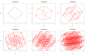
So I wrote the code (it’s only around 50 lines, and took around 30 minutes to write and debug), and running it produces plots like these:

Hypercubes in dimensions 2, 3, 4, 5, 6 and 7
Hypercubes

I’ve appended the code below, as it illustrates a lot of basic R programming concepts. Essentially, the idea is to use vectors and matrices as much as possible, but not to be really obsessed about avoiding for loops if performance isn’t critical. The code isn’t commented, but it’s highly structured and easy to understand. The function makevertices creates a matrix whose columns are the vertex locations of a hypercube. The function makeedges creates a matrix whose columns give pairs of vertex indices representing the edges of the hypercube (pairs of vertices a distance of 1 apart). The function rotate picks a pair of coordinate axes at random and rotates the hypercube in that plane. The rest are obvious, and the file finishes with some example ways to call the code. As well as illustrating the basic programming concepts such as functions, vectors, matrices and matrix operations and looping, the code also illustrates several other useful concepts such as integer division and modular arithmetic, conditional execution, optional arguments, dynamically growing a matrix, randomly sampling without replacement, plotting lines, plot options, anonymous function arguments, etc.

# hypercube.R
# code to rotate arbitrary d-dimensional hypercubes

# function definitions
makevertices=function(d)
{
	numv=2^d
	vertices=matrix(0,nrow=d,ncol=numv)
	for (j in 1:numv) {
		count=j-1
		for (i in 1:d) {
			vertices[i,j]=count%%2
			count=count%/%2
		}	
	}
	vertices
}

makeedges=function(vertices)
{
	d=dim(vertices)[1]
	numv=dim(vertices)[2]
	edges=NULL
	for (j in 1:numv) {
		for (i in j:numv) {
			if (sum(abs((vertices[,i]-vertices[,j])))==1) {
				edges=cbind(edges,c(i,j))
			}
		}
	}
	edges
}

rotate=function(vertices,angle=0.2)
{
	d=dim(vertices)[1]
	axes=sort(sample(1:d,2))
	rotmat=diag(rep(1,d))
	rotmat[axes[1],axes[1]]=cos(angle)
	rotmat[axes[2],axes[1]]=sin(angle)
	rotmat[axes[1],axes[2]]=-sin(angle)
	rotmat[axes[2],axes[2]]=cos(angle)
	vertices=rotmat %*% vertices
	vertices
}

plotcube=function(vertices,edges,col=2,lwd=2)
{
	d=dim(vertices)[1]
	plot(NULL,xlim=c(-2,2),ylim=c(-2,2),main=paste(d,"-d hypercube",sep=""),xlab="x(1)",ylab="x(2)")
	for (i in 1:dim(edges)[2]) {
		lines(c(vertices[1,edges[1,i]],vertices[1,edges[2,i]]),c(vertices[2,edges[1,i]],vertices[2,edges[2,i]]),col=col,lwd=lwd)
	}
}

rotationplot=function(vertices,edges,rotations=20,...)
{
	for (count in 1:rotations) {
		vertices=rotate(vertices,...)
		plotcube(vertices,edges)
	}
}

hypercube=function(d=4,...)
{
	vertices=makevertices(d)
	edges=makeedges(vertices)
	vertices=2*vertices
	vertices=vertices-1
	rotationplot(vertices,edges,...)
}

# examples

# hypercube()
# hypercube(3)
# hypercube(4,angle=0.1)
# hypercube(5,rotations=30)

# eof