Metropolis Hastings MCMC when the proposal and target have differing support

Introduction

Very often it is desirable to use Metropolis Hastings MCMC for a target distribution which does not have full support (for example, it may correspond to a non-negative random variable), using a proposal distribution which does (for example, a Gaussian random walk proposal). This isn’t a problem at all, but on more than one occasion now I have come across students getting this wrong, so I thought it might be useful to have a brief post on how to do it right, see what people sometimes get wrong, and why, and then think about correcting the wrong method in order to make it right…

A simple example

For this post we will consider a simple target distribution, with density

Of course this is a very simple distribution, and there are many straightforward ways to simulate it directly, but for this post we will use a random walk Metropolis-Hastings (MH) scheme with standard Gaussian innovations. So, if the current state of the chain is , a proposed new value will be generated from

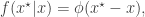
where is the standard normal density. This proposed new value is accepted with probability , where

since the standard normal density is symmetric.

Correct implementation

We can easily implement this using R as follows:

met1=function(iters)
  {
    xvec=numeric(iters)
    x=1
    for (i in 1:iters) {
      xs=x+rnorm(1)
      A=dgamma(xs,2,1)/dgamma(x,2,1)
      if (runif(1)<A)
        x=xs
      xvec[i]=x
    }
    return(xvec)
  }

We can run it, plot the results and check it against the true target with the following commands.

iters=1000000
out=met1(iters)
hist(out,100,freq=FALSE,main="met1")
curve(dgamma(x,2,1),add=TRUE,col=2,lwd=2)

If you have a slow computer, you may prefer to use iters=100000. The above code uses R’s built-in gamma density. Alternatively, we can hard-code the density as follows.

met2=function(iters)
  {
    xvec=numeric(iters)
    x=1
    for (i in 1:iters) {
      xs=x+rnorm(1)
      A=xs*exp(-xs)/(x*exp(-x))
      if (runif(1)<A)
        x=xs
      xvec[i]=x
    }
    return(xvec)
  }

We can run this code using the following commands, to verify that it does work as expected.

out=met2(iters)
hist(out,100,freq=FALSE,main="met2")
curve(dgamma(x,2,1),add=TRUE,col=2,lwd=2)

However, there is a potential problem with the above code that we have got away with in this instance, which often catches people out. We have hard-coded the density for without checking the sign of . Here we get away with it as a negative proposal will lead to a negative acceptance ratio that we will reject straight away. This is not always the case (consider, for example, a distribution). So really we should check the sign of and reject immediately if is not within the support of the target.

Although this problem often catches people out, it tends not to be a big issue in practice, as it typically leads to an obviously incorrect sampler, or a sampler which crashes, and is relatively simple to debug and fix.

An incorrect sampler

The problem I want to focus on here is more subtle, but closely related. It is clear that any should be rejected. With the above code, such values are indeed rejected, and the sampler advances to the next iteration. However, in more complex samplers, where an update like this might be one tiny part of a massive sampler with a very high-dimensional state space, it seems like a bit of a "waste" of a MH move to just propose a negative value, throw it away, and move on. Evidently, it seems tempting, therefore, to keep on sampling values until a non-negative value is obtained, and then evaluate the acceptance ratio and decide whether or not to accept. We could code up this sampler as follows.

met3=function(iters)
  {
    xvec=numeric(iters)
    x=1
    for (i in 1:iters) {
      repeat {
        xs=x+rnorm(1)
        if (xs>0)
          break
      }
      A=xs*exp(-xs)/(x*exp(-x))
      if (runif(1)<A)
        x=xs
      xvec[i]=x
    }
    return(xvec)
  }

As reasonable as this idea may at first seem, it does not lead to a sampler having the desired target, as can be verified using the following commands.

out=met3(iters)
hist(out,100,freq=FALSE,main="met3")
curve(dgamma(x,2,1),add=TRUE,col=2,lwd=2)

So, this sampler seems to be sampling something close to the desired target, but not the same. This raises a couple of questions. First and most important, can we fix this sampler so that it does sample the correct target (yes), and second, can we figure out what target density the incorrect sampler is actually sampling (again, yes)? Let’s start with the issue of how to fix the sampler, as this will also help us to understand what the incorrect sampler is doing.

Fixing the truncated sampler

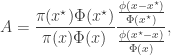
By repeatedly sampling from the proposal until we obtain a non-negative value, we are actually implementing a rejection sampler for sampling from the proposal distribution truncated at zero. This is a perfectly reasonable proposal distribution, so we can use it provided that we use the correct MH acceptance ratio. Now, the truncated density has the same density as the untruncated density, apart from the differing support and a normalising constant. Indeed, this may be why people often assume this method will work, because normalising constants often don’t matter in MH schemes. However, the normalising constant only doesn’t matter if it is independent of the state, and here it is not… Explicitly, we have

Including the normalising constant we have

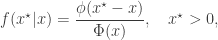
where is the standard normal CDF. Consequently, the correct acceptance ratio to use with this proposal is

where we see that the normalising constants do not cancel out. We can modify the previous sampler to use the correct acceptance ratio as follows.

met4=function(iters)
  {
    xvec=numeric(iters)
    x=1
    for (i in 1:iters) {
      repeat {
        xs=x+rnorm(1)
        if (xs>0)
          break
      }
      A=xs*exp(-xs)/(x*exp(-x))
      A=A*pnorm(x)/pnorm(xs)
      if (runif(1)<A)
        x=xs
      xvec[i]=x
    }
    return(xvec)
  }

We can verify that this sampler gives leads to the correct target with the following commands.

out=met4(iters)
hist(out,100,freq=FALSE,main="met4")
curve(dgamma(x,2,1),add=TRUE,col=2,lwd=2)

So, truncating the proposal at zero is fine, provided that you modify the acceptance ratio accordingly.

What does the incorrect sampler target?

Now that we understand why the naive truncated sampler was wrong and how to fix it, we can, out of curiosity, wonder what distribution that sampler actually targets. Now we understand what proposal we are actually using, we can re-write the acceptance ratio as

from which it is clear that the actual target of this chain is

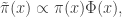
or

The constant of proportionality is not immediately obvious, but is tractable, and turns out to be a nice undergraduate exercise in integration by parts, leading to

We can verify this using the following commands.

out=met3(iters)
hist(out,100,freq=FALSE,main="met3")
curve(dgamma(x,2,1)*pnorm(x)*2*sqrt(2*pi)/(sqrt(2*pi)+2),add=TRUE,col=3,lwd=2)

Now we know the actual target of the incorrect sampler, we can compare it with the correct target as follows.

curve(dgamma(x,2,1),0,10,col=2,lwd=2,main="Densities")
curve(dgamma(x,2,1)*pnorm(x)*2*sqrt(2*pi)/(sqrt(2*pi)+2),add=TRUE,col=3,lwd=2)

So we see that the distributions are different, but not so different that one would immediate suspect an error on the basis of a sample of output. This makes it a difficult bug to track down.

Summary

There is no problem in principle using a proposal with full support for a target with limited support in MH algorithms. However, it is important to check whether a proposed value is within the support of the target and reject the proposed move if it is not. If you are concerned that such a scheme might be inefficient, it is possible to use a truncated proposal provided that you modify the MH acceptance ratio to include the relevant normalisation constants. If you don’t modify the acceptance probability, you will get a sampler which targets the wrong distribution, but it will often be quite similar to the correct target, making it a difficult bug to spot and track down.